90+% accuracy? Made possible with Transfer Learning.
Last week, you’ve seen how data augmentation can squeeze an extra couple of percent accuracy from your TensorFlow models. We only scratched the surface compared to what you’ll see today. We’ll finally get above 90% accuracy on the validation set with a pretty straightforward approach.
You’ll also see what happens to the validation accuracy if we scale down the amount of training data by a factor of 20. Spoiler alert - it will remain unchanged.
Don’t feel like reading? Watch my video instead:
You can download the source code on GitHub.
What is Transfer Learning in TensorFlow?
Writing neural network model architectures from scratch involves a lot of guesswork. How many layers? How many nodes per layer? What activation function to use? Regularization? You won’t run out of questions any time soon.
Transfer learning takes a different approach. Instead of starting from scratch, you take an existing neural network model that has been trained by someone really smart on an enormous dataset with far superior hardware than you have at home. These networks can have hundreds of layers, unlike our 2-block CNN implemented weeks ago.
Long story short - the deeper you go into the network, the more sophisticated features you’ll extract.
The entire transfer learning process boils down to 3 steps:
- Take a pretrained network - For example, take a VGG, ResNet, or EfficientNet architecture that’s been trained on millions of images to detect 1000 classes.
- Cut the head of the model - Exclude the last few layers of a pretrained model and replace them with your own. For example, our dogs vs. cats dataset has two classes, and the final classification layer needs to resemble that.
- Fine-tune the final layers - Train the network on your dataset to adjust the classifier. Weights of the pretrained model are frozen, meaning they won’t update as you train the model.
What all of this boils down to is that transfer learning allows you to get drastically better results with less data. Our custom 2-block architecture gave only 76% accuracy on the validation set. Transfer learning will skyrocket it to above 90%.
Getting Started - Library and Dataset Imports
We’ll use the Dogs vs. Cats dataset from Kaggle. It’s licensed under the Creative Commons License, which means you can use it for free:

Image 1 — Dogs vs. Cats dataset (image by author)
The dataset is fairly large — 25,000 images distributed evenly between classes (12,500 dog images and 12,500 cat images). It should be big enough to train a decent image classifier. The only problem is — it’s not structured for deep learning out of the box. You can follow my previous article to create a proper directory structure, and split it into train, test, and validation sets:
TensorFlow for Computer Vision — Top 3 Prerequisites for Deep Learning Projects
You should also delete the train/cat/666.jpg and train/dog/11702.jpg images as they’re corrupted, and your model will fail to train with them.
Once done, you can proceed with the library imports. We’ll only need Numpy and TensorFlow today. Other imports are here to get rid of unnecessary warning messages:
import os
os.environ['TF_CPP_MIN_LOG_LEVEL'] = '3'

import warnings
warnings.filterwarnings('ignore')

import numpy as np
import tensorflow as tf
We’ll have to load training and validation data from different directories throughout the article. The best practice is to declare a function for loading the images and data augmentation:
def init_data(train_dir: str, valid_dir: str) -> tuple:
    train_datagen = tf.keras.preprocessing.image.ImageDataGenerator(
        rescale=1/255.0,
        rotation_range=20,
        width_shift_range=0.2,
        height_shift_range=0.2,
        shear_range=0.2,
        zoom_range=0.2,
        horizontal_flip=True,
        fill_mode='nearest'
    )
    valid_datagen = tf.keras.preprocessing.image.ImageDataGenerator(
        rescale=1/255.0
    )

    train_data = train_datagen.flow_from_directory(
        directory=train_dir,
        target_size=(224, 224),
        class_mode='categorical',
        batch_size=64,
        seed=42
    )
    valid_data = valid_datagen.flow_from_directory(
        directory=valid_dir,
        target_size=(224, 224),
        class_mode='categorical',
        batch_size=64,
        seed=42
    )

    return train_data, valid_data
Let’s now load our dogs and cats dataset:
train_data, valid_data = init_data(
    train_dir='data/train/',
    valid_dir='data/validation/'
)
Here’s the output you should see:
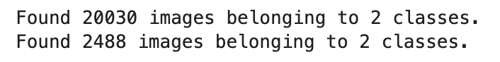
Image 2 - Number of training and validation images (image by author)
Is 20K training images an overkill for transfer learning? Probably, but let’s see how accurate of a model can we get.
Transfer Learning with TensorFlow in Action
With transfer learning, we’re basically loading a huge pretrained model without the top classification layer. That way, we can freeze the learned weights and only add the output layer to match our dataset.
For example, most pretrained models were trained on the ImageNet dataset which has 1000 classes. We only have two (cat and dog), so we’ll need to specify that.
That’s where the build_transfer_learning_model() function comes into play. It has a single parameter - base_model - which represents the pretrained architecture. First, we’ll freeze all the layers in that model, and then build a Sequential model from it by adding a couple of custom layers. Finally, we’ll compile the model using the usual suspects:
def build_transfer_learning_model(base_model):
    # `base_model` stands for the pretrained model
    # We want to use the learned weights, and to do so we must freeze them
    for layer in base_model.layers:
        layer.trainable = False

    # Declare a sequential model that combines the base model with custom layers
    model = tf.keras.Sequential([
        base_model,
        tf.keras.layers.GlobalAveragePooling2D(),
        tf.keras.layers.BatchNormalization(),
        tf.keras.layers.Dropout(rate=0.2),
        tf.keras.layers.Dense(units=2, activation='softmax')
    ])

    # Compile the model
    model.compile(
        loss='categorical_crossentropy',
        optimizer=tf.keras.optimizers.Adam(),
        metrics=['accuracy']
    )

    return model
Now the fun part begins. Import the VGG16 architecture from TensorFlow and specify it as a base model to our build_transfer_learning_model() function. The include_top=False parameter means we don’t want the top classification layer, as we’ve declared our own. Also, note how the input_shape was set to resemble the shapes of our images:
# Let's use a simple and well-known architecture - VGG16
from tensorflow.keras.applications.vgg16 import VGG16

# We'll specify it as a base model
# `include_top=False` means we don't want the top classification layer
# Specify the `input_shape` to match our image size
# Specify the `weights` accordingly
vgg_model = build_transfer_learning_model(
    base_model=VGG16(include_top=False, input_shape=(224, 224, 3), weights='imagenet')
)

# Train the model for 10 epochs
vgg_hist = vgg_model.fit(
    train_data,
    validation_data=valid_data,
    epochs=10
)
Here’s the output after training the model for 10 epochs:
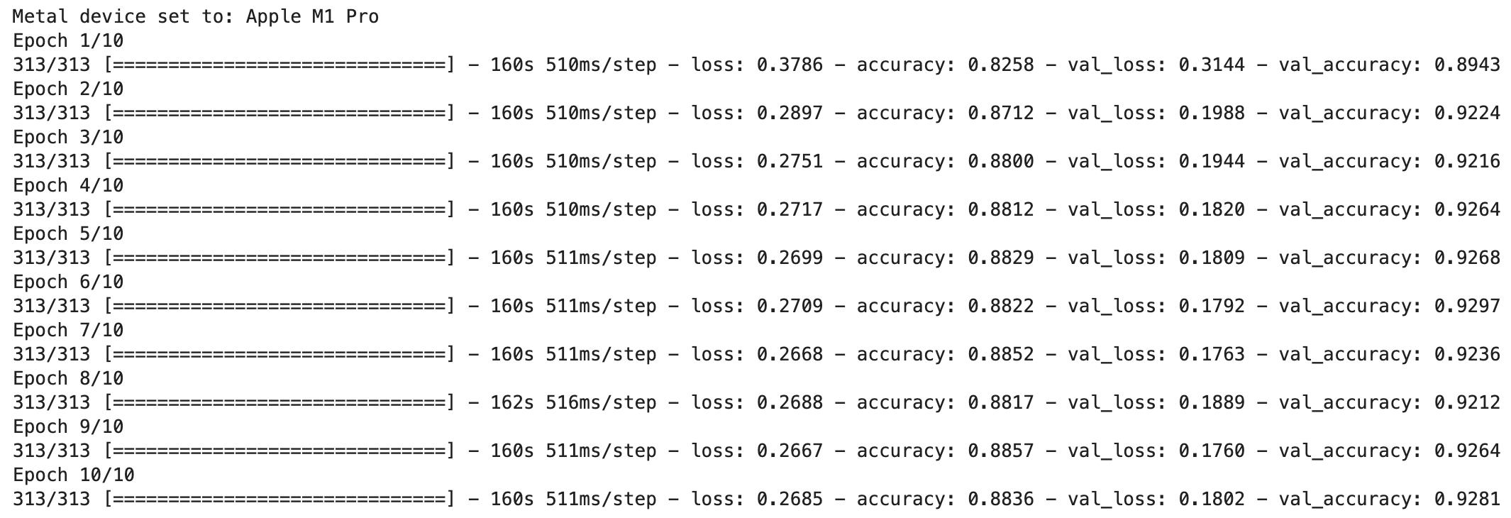
Image 3 - VGG16 model on 20K training images after 10 epochs (image by author)
Now that’s something to write home about - 93% validation accuracy without even thinking about the mode architecture. The real beauty of transfer learning lies in the amount of data needed to train accurate models, which is much less than with custom architectures.
How much less? Let’s scale our dataset down 20 times to see what happens.
Transfer Learning on a 20X Smaller Subset
We want to see if reducing the dataset size negatively affects the predictive power. Create a new directory structure for training and validation images. Images will be stored inside the data_small folder, but feel free to rename it to anything else:
import random
import pathlib
import shutil

random.seed(42)


dir_data = pathlib.Path.cwd().joinpath('data_small')
dir_train = dir_data.joinpath('train')
dir_valid = dir_data.joinpath('validation')

if not dir_data.exists(): dir_data.mkdir()
if not dir_train.exists(): dir_train.mkdir()
if not dir_valid.exists(): dir_valid.mkdir()

for cls in ['cat', 'dog']:
    if not dir_train.joinpath(cls).exists(): dir_train.joinpath(cls).mkdir()
    if not dir_valid.joinpath(cls).exists(): dir_valid.joinpath(cls).mkdir()
Here’s the command you can use to print the directory structure:
!ls -R data_small | grep ":$" | sed -e 's/:$//' -e 's/[^-][^\/]*\//--/g' -e 's/^/ /' -e 's/-/|/'
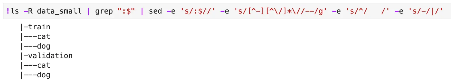
Image 4 - Directory structure (image by author)
Copy a sample of the images to the new folder. The copy_sample() function takes n images from the src_folder and copies them to the tgt_folder. By default, we’ll set n to 500:
def copy_sample(src_folder: pathlib.PosixPath, tgt_folder: pathlib.PosixPath, n: int = 500):
    imgs = random.sample(list(src_folder.iterdir()), n)

    for img in imgs:
        img_name = str(img).split('/')[-1]

        shutil.copy(
            src=img,
            dst=f'{tgt_folder}/{img_name}'
        )
Let’s now copy the training and validation images. For the validation set, we’ll copy only 100 images per class:
# Train - cat
copy_sample(
    src_folder=pathlib.Path.cwd().joinpath('data/train/cat/'),
    tgt_folder=pathlib.Path.cwd().joinpath('data_small/train/cat/'),
)

# Train - dog
copy_sample(
    src_folder=pathlib.Path.cwd().joinpath('data/train/dog/'),
    tgt_folder=pathlib.Path.cwd().joinpath('data_small/train/dog/'),
)

# Valid - cat
copy_sample(
    src_folder=pathlib.Path.cwd().joinpath('data/validation/cat/'),
    tgt_folder=pathlib.Path.cwd().joinpath('data_small/validation/cat/'),
    n=100
)

# Valid - dog
copy_sample(
    src_folder=pathlib.Path.cwd().joinpath('data/validation/dog/'),
    tgt_folder=pathlib.Path.cwd().joinpath('data_small/validation/dog/'),
    n=100
)
Use the following commands to print the number of images in each folder:
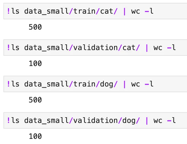
Image 5 - Number of training and validation images per class (image by author)
Finally, call init_data() function to load images from the new source:
train_data, valid_data = init_data(
    train_dir='data_small/train/',
    valid_dir='data_small/validation/'
)
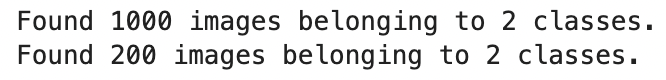
Image 6 - Number of training and validation images in the smaller subset (image by author)
There are 1000 training images in total. It will be interesting to see if we can get a decent model out of a dataset this small. We’ll keep the model architecture identical, but train for more epochs just because the dataset is smaller. Also, we can afford to train for longer since the training time per epoch is reduced:
vgg_model = build_transfer_learning_model(
    base_model=VGG16(include_top=False, input_shape=(224, 224, 3), weights='imagenet')
)

vgg_hist = vgg_model.fit(
    train_data,
    validation_data=valid_data,
    epochs=20
)
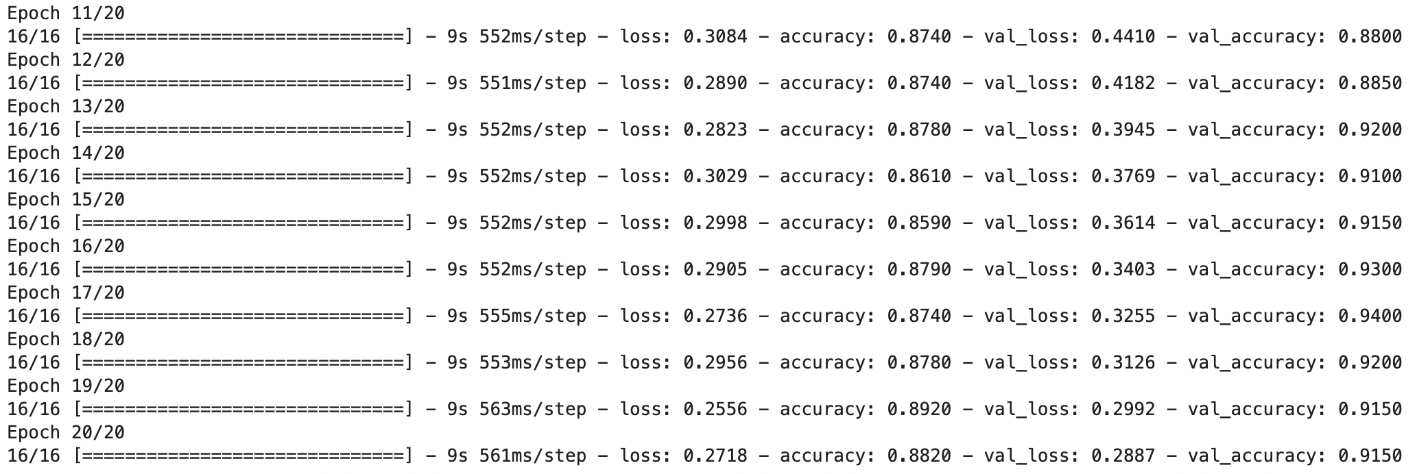
Image 7 - Training results of the last 10 epochs (image by author)
And would you look at that - we got roughly the same validation accuracy as with the model trained on 20K images, which is amazing.
That’s where the true power of transfer learning lies. You don’t always have access to huge datasets, so it’s amazing to see we can build something this accurate with such limited data.
Conclusion
To recap, transfer learning should be your go-to approach when building image classification models. You don’t need to think about the architecture, as someone already did that for you. You don’t need to have a huge dataset, as someone already trained a general-purpose model on millions of images. Finally, you don’t need to worry about poor performance most of the time, unless your dataset is highly specialized.
The only thing you need to do is to choose a pre-trained architecture. We opted for VGG16 today, but I encourage you to experiment with ResNet, MobileNet, EfficientNet, and others.
Here’s another homework assignment you can do - use both models trained today to predict the entire test set. How do the accuracies compare? Please let me know.
Stay connected
- Sign up for my newsletter
- Subscribe on YouTube
- Connect on LinkedIn