Small dataset? No problem - expand it with data augmentation and increase the model’s predictive power.
Last week, you saw that more complex models don’t increase the predictive power. In fact, we ended up with an even worse image classifier! What can you do to bring the accuracy up? Well, a couple of things, but data augmentation is a great place to start.
Today you’ll learn all about data augmentation with TensorFlow, what it does to an image dataset, why it improves predictive performance, and how to use it on custom datasets. So without much ado, let’s dive straight in!
Don’t feel like reading? Watch my video instead:
You can download the source code on GitHub.
Getting Started - Data and Library Imports
We’ll use the Dogs vs. Cats dataset from Kaggle. It’s licensed under the Creative Commons License, which means you can use it for free:

Image 1 — Dogs vs. Cats dataset (image by author)
The dataset is fairly large — 25,000 images distributed evenly between classes (12,500 dog images and 12,500 cat images). It should be big enough to train a decent image classifier. The only problem is — it’s not structured for deep learning out of the box. You can follow my previous article to create a proper directory structure, and split it into train, test, and validation sets:
TensorFlow for Computer Vision — Top 3 Prerequisites for Deep Learning Projects
You should also delete the train/cat/666.jpg and train/dog/11702.jpg images as they’re corrupted, and your model will fail to train with them.
Once done, you can proceed with the library imports. We’ll only need a few today - Numpy, TensorFlow, Matplotlib, and PIL. The below snippet imports them all, and also declares a function for displaying images:
import numpy as np
import tensorflow as tf
from tensorflow.keras import layers
import matplotlib.pyplot as plt
from PIL import Image


def plot_image(img: np.array):
    plt.figure(figsize=(6, 6))
    plt.imshow(img, cmap='gray');
We’ll now use that function to load a sample image from the training set:
img = Image.open('data/train/cat/1.jpg')
img = np.array(img)
plot_image(img=img)
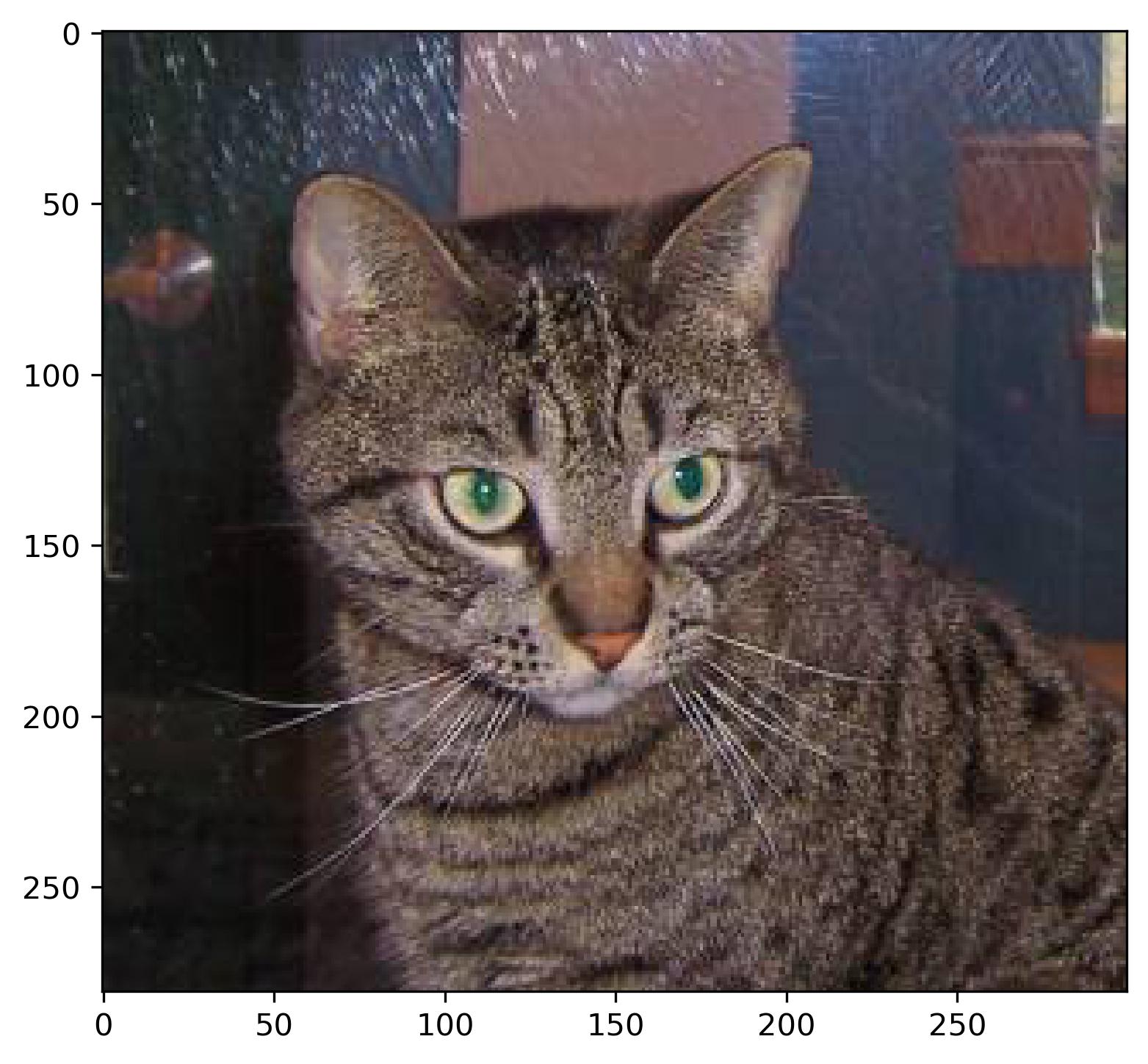
Image 2 - A sample image from the training set (image by author)
That’s all we need to get started with data augmentation, so let’s do that next.
Data Augmentation with TensorFlow in Action
Put simply, data augmentation is a technique used to increase the amount of data by modifying the data that already exists. By doing so, a predictive model is exposed to more data than before, and in theory, should learn to model it better. At the very least, you should expect a few percent increase in accuracy (or any other metric) if you have a decent dataset in the first place.
Data augmentation with TensorFlow works by applying different transformations randomly to an image dataset. These transformations include horizontal/vertical flipping, rotation, zoom, width/height shifts, shear, and so on. Refer to the official documentation for a full list of available options.
We’ll start by declaring a model which resizes an image to 224x224 pixels and rescales its underlying matrix to a 0-1 range. It’s not a common practice to declare a model for data augmentation, but you’ll be able to see exactly what’s going on this way:
resize_and_scale = tf.keras.Sequential([
    layers.Resizing(224, 224),
    layers.Rescaling(1./255)
])

res = resize_and_scale(img)
plot_image(img=res)

Image 3 - Cat image after resizing and rescaling (image by author)
Nothing much happened here, but you can verify the transformation was applied by comparing the axis ticks on Image 2 and Image 3. You can also print the minimum and maximum values of the image matrix before and after the transformation, but I’ll leave that up to you.
Let’s spice things up by adding random horizontal flips and random rotations. A RandomFlip layer flips the image horizontally, vertically, or both, depending on the mode parameter. A RandomRotation layer rotates the image by some factor. For example, if a factor is set to 0.2, a rotation degree is calculated as 0.2 * 2PI:
augmentation = tf.keras.Sequential([
    layers.RandomFlip(mode='horizontal'),
    layers.RandomRotation(factor=0.2)
])

res = augmentation(img)
plot_image(img=res)
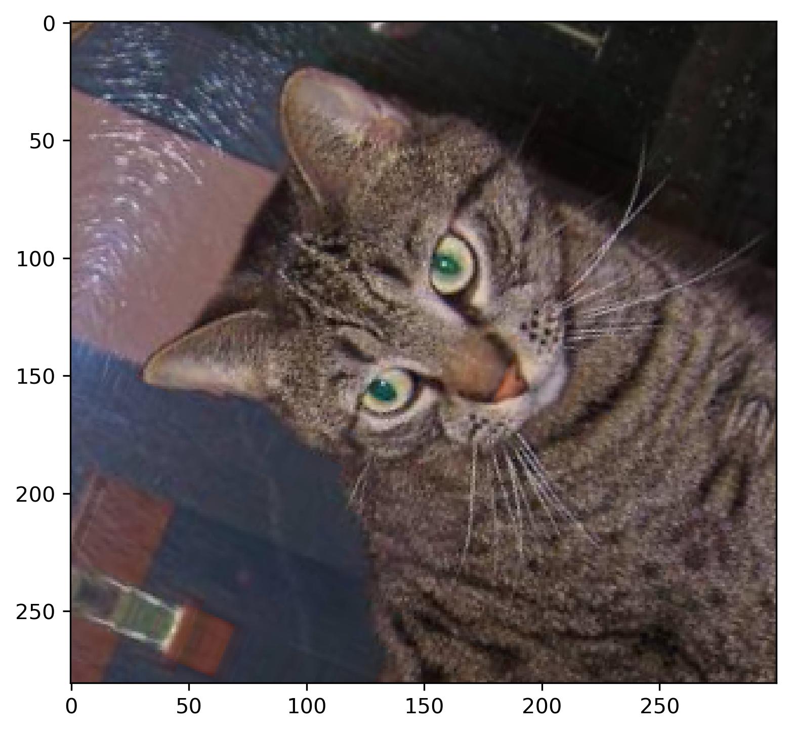
Image 4 - Cat image after flipping and rotating (image by author)
It’s still the same image, but definitely with more variety added to it. We’ll spice things up even more with zooming and translating. A RandomZoom layer does what the name suggests - zooms image based on a factor. For example, a factor of 0.2 means 20%. A RandomTranslation layer shifts the image vertically or horizontally, depending on the two corresponding factors. The height_factor parameter represents the vertical shift, and width_factor represents the horizontal shift:
augmentation = tf.keras.Sequential([
    layers.RandomFlip(mode='horizontal_and_vertical'),
    layers.RandomRotation(factor=0.2),
    layers.RandomZoom(height_factor=0.2, width_factor=0.2),
    layers.RandomTranslation(height_factor=0.2, width_factor=0.2)
])

res = augmentation(img)
plot_image(img=res)
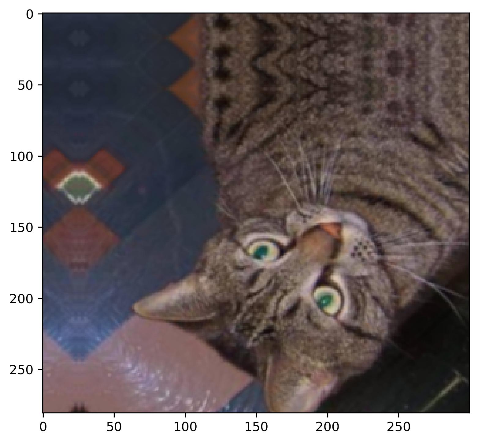
Image 5 - Cat image after flipping, rotating, zooming, and translating (image by author)
The images are getting weirder as we add more transformations, but we still have no problem classifying them as a cat. The transformations you’ve seen are random, and to verify this claim, we can make a 3x3 plot showing results of 9 random transformations:
plt.figure(figsize=(10, 10))

for i in range(9):
    img_aug = augmentation(img)
    ax = plt.subplot(3, 3, i + 1)
    plt.imshow(img_aug)
    plt.axis('off')
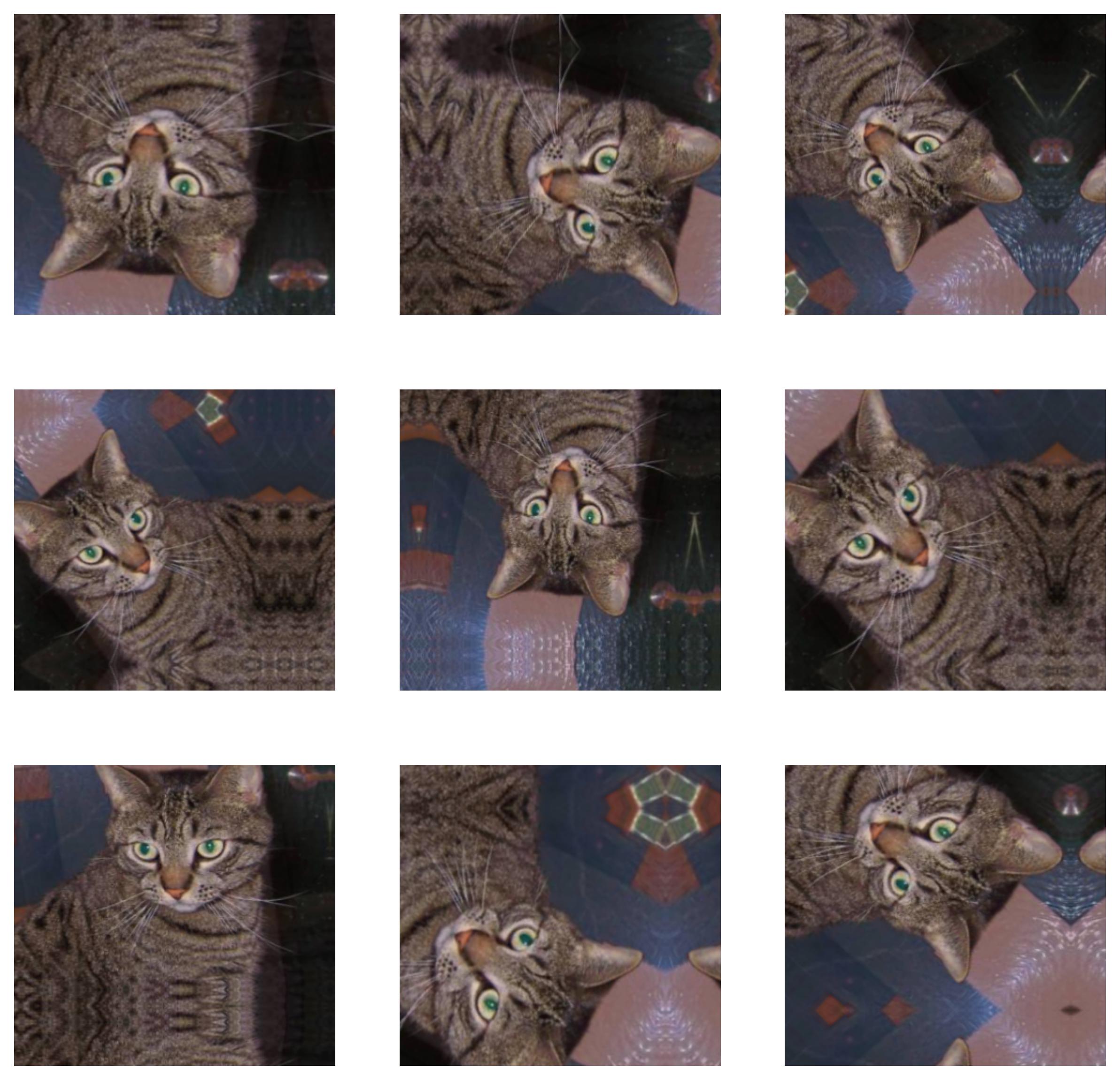
Image 6 - 9 random transformations applied to the same image (image by author)
Some of them make sense, while others don’t - but the image itself isn’t more difficult to classify. Next, let’s see how to handle data augmentation with TensorFlow’s ImageDataGenerator.
Data Augmentation with TensorFlow’s ImageDataGenerator
You now know what individual transformations do to an image, but it isn’t common to write data augmentation as a separate Sequential model. More often than not, you’ll apply the transformations when loading the image data with TensorFlow’s ImageDataGenerator classes.
Keep in mind - You should only augment the training data.
Doing data augmentation this way is easier. The following code snippet applies rescaling, rotation, shift, shear, zoom, and horizontal flip to the training set, and only rescales the validation set. The fill_mode parameter tells TensorFlow how to handle points outside the image boundaries which were made as a side effect of some transformations.
train_datagen = tf.keras.preprocessing.image.ImageDataGenerator(
    rescale=1/255.0,
    rotation_range=20,
    width_shift_range=0.2,
    height_shift_range=0.2,
    shear_range=0.2,
    zoom_range=0.2,
    horizontal_flip=True,
    fill_mode='nearest'
)

valid_datagen = tf.keras.preprocessing.image.ImageDataGenerator(
    rescale=1/255.0
)
How can we know if this worked? Simply - we’ll visualize a single batch of images. First, we have to call the flow_from_directory() function to specify the batch size, among other parameters:
train_data = train_datagen.flow_from_directory(
    directory='data/train/',
    target_size=(224, 224),
    class_mode='categorical',
    batch_size=64,
    seed=42
)
The train_data is now a Python generator object, so calling next() on it returns the first batch. Here’s how to extract it and print the shape of its elements:
first_batch = train_data.next()
first_batch[0].shape, first_batch[1].shape
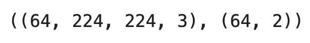
Image 7 - Shape of the first batch (image by author)
In a nutshell, we have 64 images, each being 224 pixels wide, 224 pixels tall, and with 3 color channels. The second element represents the labels. We have 64 of these in one-hot encoded format (cat = [1, 0], dog = [0, 1]).
Use the following function to visualize a batch of 64 images in an 8x8 grid:
def visualize_batch(batch: tf.keras.preprocessing.image.DirectoryIterator):
    n = 64
    num_row, num_col = 8, 8
    fig, axes = plt.subplots(num_row, num_col, figsize=(3 * num_col, 3 * num_row))

    for i in range(n):
        img = np.array(batch[0][i] * 255, dtype='uint8')
        ax = axes[i // num_col, i % num_col]
        ax.imshow(img)

    plt.tight_layout()
    plt.show()


visualize_batch(batch=first_batch)
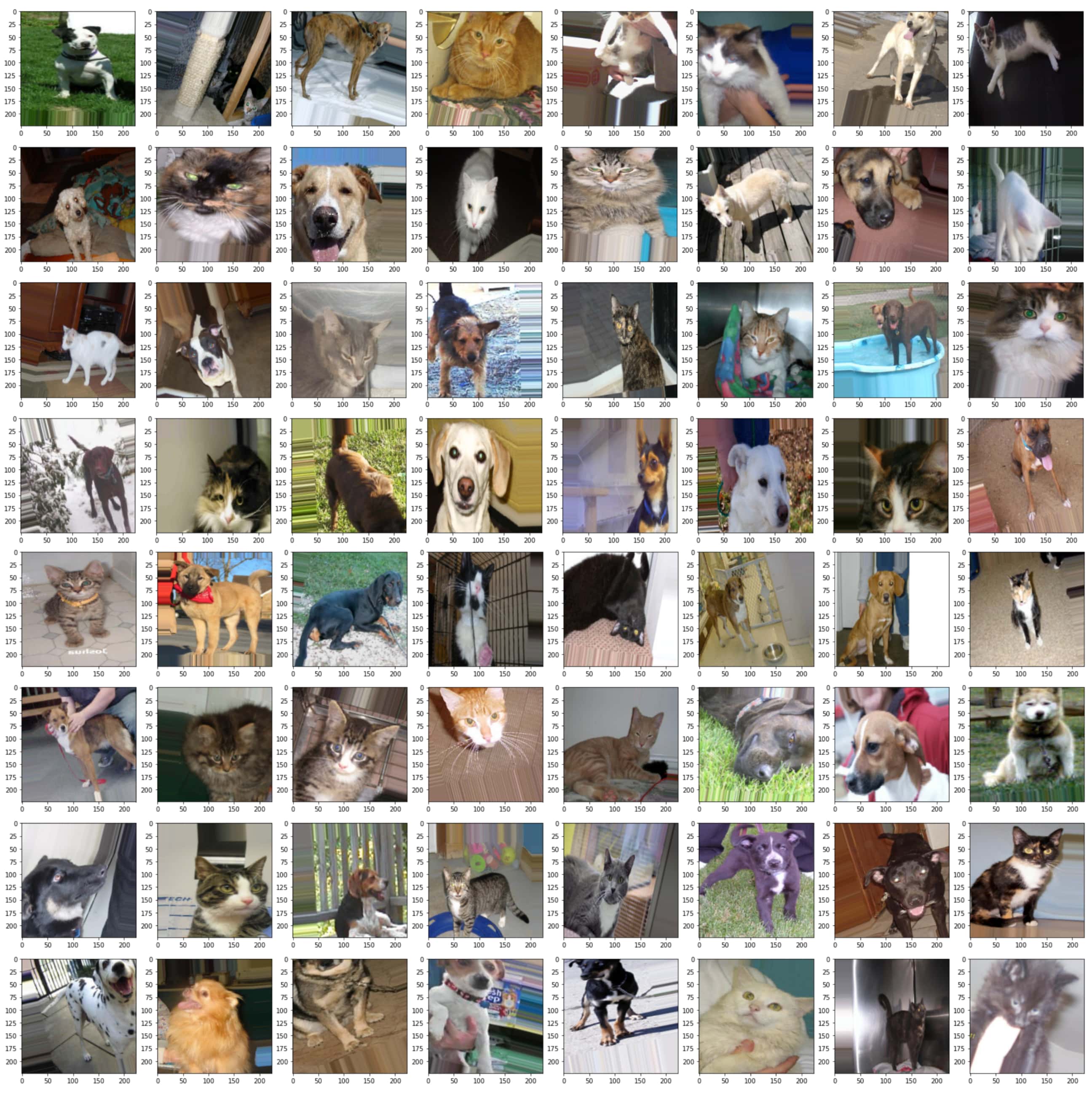
Image 8 - A single batch of 64 images (image by author)
We definitely have some weird ones, but overall, data augmentation is doing a decent job by adding variety to our dataset. As a final step, we’ll load in both training and validation images:
train_data = train_datagen.flow_from_directory(
    directory='data/train/',
    target_size=(224, 224),
    class_mode='categorical',
    batch_size=64,
    seed=42
)

valid_data = valid_datagen.flow_from_directory(
    directory='data/validation/',
    target_size=(224, 224),
    class_mode='categorical',
    batch_size=64,
    seed=42
)
That’s all we need to train the model. Fingers crossed it outperforms the previous one!
Model Training - Can Data Augmentation with TensorFlow Improve Accuracy?
We’ll use the same model architecture we used when first training an image classifier with convolutional networks. It achieved around 75% accuracy on the validation set. Data augmentation should hopefully kick things up a notch.
Here’s the model training code - it has two convolutional/pooling blocks followed by a single dense layer and an output layer:
model = tf.keras.Sequential([
    layers.Conv2D(filters=32, kernel_size=(3, 3), input_shape=(224, 224, 3), activation='relu'),
    layers.MaxPool2D(pool_size=(2, 2), padding='same'),
    layers.Conv2D(filters=32, kernel_size=(3, 3), activation='relu'),
    layers.MaxPool2D(pool_size=(2, 2), padding='same'),
    layers.Flatten(),
    layers.Dense(128, activation='relu'),
    layers.Dense(2, activation='softmax')
])

model.compile(
    loss=tf.keras.losses.categorical_crossentropy,
    optimizer=tf.keras.optimizers.Adam(),
    metrics=[tf.keras.metrics.BinaryAccuracy(name='accuracy')]
)

history = model.fit(
    train_data,
    validation_data=valid_data,
    epochs=10
)
Note: I’m facing some GPU issues so the model was trained on the CPU, hence the long training time. My RTX 3060Ti usually goes over an epoch in 22 seconds.
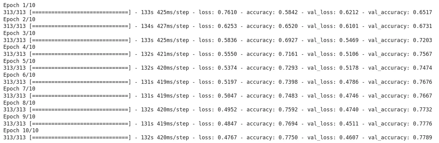
Image 9 - Model training results (image by author)
Data augmentation increased the validation accuracy by almost 3%! It’s definitely a step in the right direction, but we can improve it even further. How? With transfer learning. You’ll learn all about it in the following article.
Conclusion
And there you have it - how to easily squeeze an extra couple of percent accuracy from your models. Data augmentation is a powerful tool when building image classifiers, but be careful with it. If it doesn’t make sense to flip the image vertically, don’t do it. For example, flipping traffic signs horizontally and vertically won’t help you with classification. These are usually read from top to bottom and from left to right. The same goes for any other transformation.
I’m excited about the upcoming transfer learning articles, as it is a go-to approach for building highly-accurate models with limited data. Stay tuned to learn all about it!
Stay connected
- Sign up for my newsletter
- Subscribe on YouTube
- Connect on LinkedIn