
Combine Convolutions and Pooling if you want a decent from-scratch image classifier
You saw last week that vanilla Artificial neural networks are terrible for classifying images. And that’s expected, as they have no idea about 2D relationships between pixels. That’s where convolutions come in — a go-to approach for finding patterns in image data.
Want to hear the good news? Today you’ll learn the basics behind convolutional and pooling layers, and you’ll also train and evaluate your first real image classifier. It’s gonna be a long one. A cup of strong coffee is recommended.
As always, we’ll keep the theory light and hands-on parts strong. Feel free to watch my video if you don’t feel like reading:
You can download the source code on GitHub.
Introduction to Convolutions and Pooling
We can’t discuss Convolutional neural networks before skimming over convolution and pooling theory first. Both are simpler than you think, but extremely capable in image classification.
Convolutions
Convolutional neural networks are a special type of neural network used for image classification. At the heart of any convolutional neural network lies convolution, an operation highly specialized at detecting patterns in images.
Convolutional layers require you to specify the number of filters. Think of these as a number of pattern detectors. Early convolutional layers detect basic patterns, such as edges, corners, and so on. Specialized patterns are detected at later convolutional layers, such as dog ears or cat paws, depending on the dataset.
A single filter is just a small matrix (usually rectangular). It’s your task to decide on the number of rows and columns, but 3x3 or 5x5 are good starting points. Values inside the filter matrix are initialized randomly. The task of a neural network is to learn the optimal values for the filter matrix, given your specific dataset.
Let’s take a look at a convolution operation in action. We have a 5x5 image and a 3x3 filter. The filter slides (convolves) over every 3x3 set of pixels in the image, and calculates an element-wise multiplication. The multiplication results are then summed:
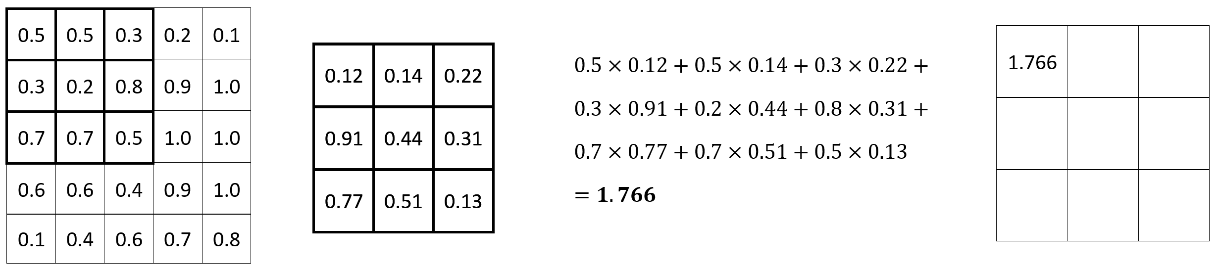
Image 1 — Convolution operation (1) (image by author)
The process is repeated for every set of 3x3 pixels. Here’s the calculation for the following set:
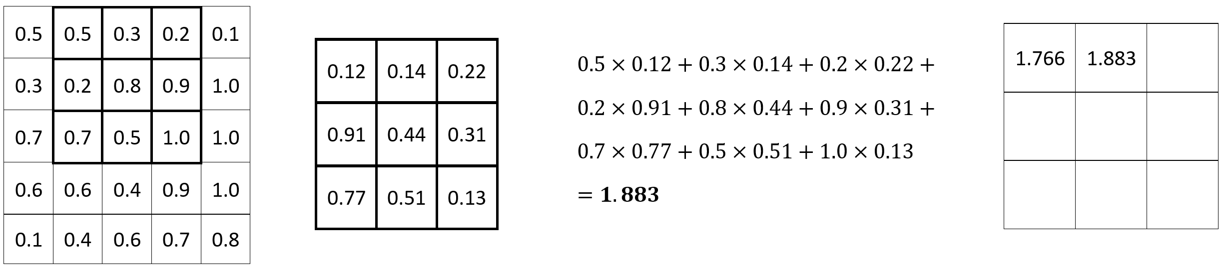
Image 2 — Convolution operation (2) (image by author)
The process is repeated until the final set of 3x3 pixels is reached:
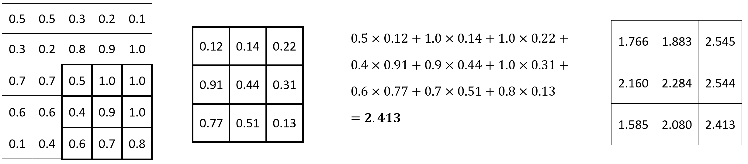
Image 3 — Convolution operation (3) (image by author)
From here, you can flatten the result, pass it into another convolutional layer, or, most commonly, pass it through a pooling layer.
Pooling
The pooling operation usually follows the convolution. Its task is to reduce the dimensionality of the result coming in from the convolutional layer by keeping what’s relevant and discarding the rest.
The process is simple — you define an n x n region and stride size. The n x n region represents a small matrix on which pooling is performed. The stride represents the number of pixels to the right (or bottom) the pooling operation moves after completing a single step.
The most common type of pooling is Max Pooling, the most common region size is 2x2, and the most common stride size is 2. This means we’re looking at a small matrix of 2x2 pixels at a time and keeping the largest value only. Here’s an example:
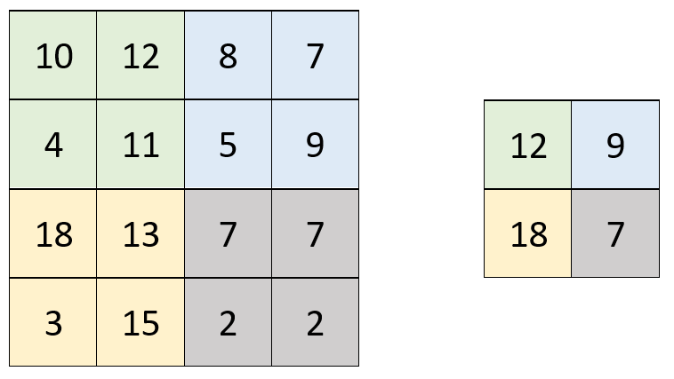
Image 4 — Max Pooling operation (image by author)
Simple, isn’t it? You don’t have to take the maximum value. Another common type of pooling is Average Pooling, and it does what the name suggests. Max Pooling is used more often, so we’ll stick to it throughout the article.
To summarize, max pooling reduces the number of parameters by keeping only the pixels with the highest values (most activated ones) and disregarding everything else.
You now know the basics behind these two operations, so let’s implement them next. We’ll dive much deeper into how convolutions and pooling work in the following article.
Dataset Used and Data Preprocessing
We’ll use the Dogs vs. Cats dataset from Kaggle. It’s licensed under the Creative Commons License, which means you can use it for free:

Image 5 — Dogs vs. Cats dataset (image by author)
The dataset is fairly large — 25,000 images distributed evenly between classes (12,500 dog images and 12,500 cat images). It should be big enough to train a decent image classifier. The only problem is — it’s not structured for deep learning out of the box. You can follow my previous article to create a proper directory structure, and split it into train, test, and validation sets:
TensorFlow for Computer Vision — Top 3 Prerequisites for Deep Learning Projects
Before proceeding, please delete the following images:
data/train/cat/666.jpgdata/train/dog/11702.jpg
These caused errors during training as they are corrupted, so it’s best to get rid of them altogether.
How to Normalize Image Data
Let’s get the library imports out of the way. You won’t need much today:
import os
import pathlib
os.environ['TF_CPP_MIN_LOG_LEVEL'] = '2'

import numpy as np
import matplotlib.pyplot as plt
import tensorflow as tf
tf.random.set_seed(42)

from PIL import Image, ImageOps
from IPython.display import display
import warnings
warnings.filterwarnings('ignore')
So, what’s wrong with our image dataset? Let’s load a couple of images and inspect. Use the following code to load a random image from the cat folder:
img1 = Image.open('data/train/cat/1.jpg')
print(np.array(img1).shape)
display(img1)
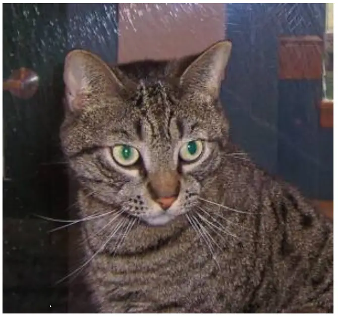
Image 6 — Sample cat image (image by author)
The above cat image is 281 pixels tall, 300 pixels wide, and has three color channels. Does the same hold for a random dog image?
img2 = Image.open('data/train/dog/0.jpg')
print(np.array(img2).shape)
display(img2)
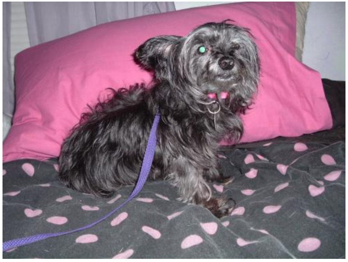
Image 7 — Sample dog image (image by author)
The dog image is 375 pixels tall, 500 pixels wide, and has 3 color channels. It’s larger than the first image, and a neural network won’t like that. It expects images (arrays) of identical sizes. We can resize them as we feed data to the model.
There’s a more urgent issue to address. The pixel values range from 0 to 255 (np.array(img2)):
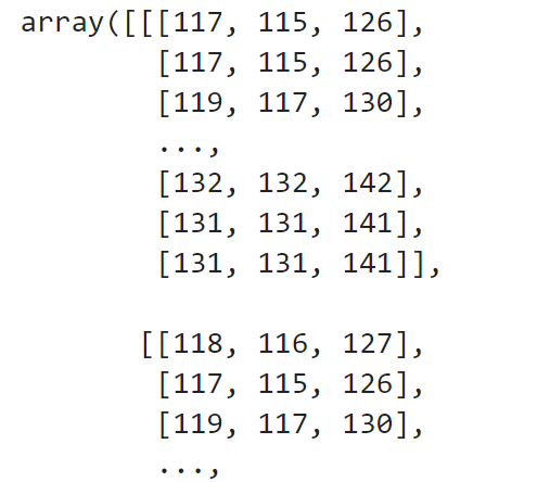
Image 8 — Image converted to array (image by author)
Neural networks prefer a range between 0 and 1. You can translate an image to that range by dividing each element with 255.0:
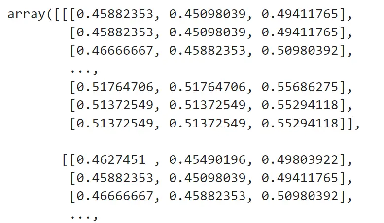
Image 9 — Image converted to an array and normalized (image by author)
You can do this step automatically with data loaders.
TensorFlow Data Loaders
The ImageDataGenerator class from TensorFlow is used to specify how the image data is generated. You can do a lot with it, but we’ll work only with rescaling today:
train_datagen = tf.keras.preprocessing.image.ImageDataGenerator(rescale=1/255.0)
valid_datagen = tf.keras.preprocessing.image.ImageDataGenerator(rescale=1/255.0)
You can use these generators to load image data from a directory. You’ll have to specify:
- Directory path— where the images are stored.
- Target size— the size to which all images will be resized to. 224x224 works well with neural networks.
- Class mode— set it to categorical, as we have two distinct image classes.
- Batch size— represents the number of images shown to a neural network at once.
- Seed— To get the same images I did.
train_data = train_datagen.flow_from_directory(
    directory='data/train/',
    target_size=(224, 224),
    class_mode='categorical',
    batch_size=64,
    seed=42
)
Here’s the output you should see:

Image 10 — Number of images found in the training directory (image by author)
There are 20,030 images in the training folder divided into two classes. The train_data variable is a Python generator object, which means you can access a single batch of images easily:
first_batch = train_data.next()
Each batch contains images and labels. Let’s check the shape of these:
first_batch[0].shape, first_batch[1].shape
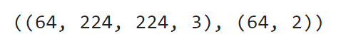
Image 11 — Shapes of batch images and labels (image by author)
A single batch contains 64 images, each being 224 pixels wide and tall and having 3 color channels. There are 64 corresponding labels. Each is an array with two elements — the probabilities of an image being a cat (index 0) and a dog (index 1).
Let’s take this one step further by visualizing a single batch.
Visualize a Single Batch of Images
You should always visualize your data. It’s the best way to spot an issue with the data loaders. Keep in mind — the images were previously rescaled to a 0–1 range. To visualize them, you have to multiply the pixel values by 255 and convert the result to integers.
The rest of the code is self-explanatory:
def visualize_batch(batch: tf.keras.preprocessing.image.DirectoryIterator):
    n = 64
    num_row, num_col = 8, 8
    fig, axes = plt.subplots(num_row, num_col, figsize=(3 * num_col, 3 * num_row))

    for i in range(n):
        img = np.array(batch[0][i] * 255, dtype='uint8')
        ax = axes[i // num_col, i % num_col]
        ax.imshow(img)

    plt.tight_layout()
    plt.show()


visualize_batch(batch=first_batch)

Image 12 — A single batch of images (image by author)
Some of these look a bit weird due to changes in the aspect ratio, but it shouldn’t be an issue. All images are now 224 pixels tall and wide, which means we’re ready to train the model.
Train a Convolutional Neural Network with TensorFlow
First things first, let’s reset our training data loader and add a loader for the validation set:
train_data = train_datagen.flow_from_directory(
    directory='data/train/',
    target_size=(224, 224),
    class_mode='categorical',
    batch_size=64,
    seed=42
)

valid_data = valid_datagen.flow_from_directory(
    directory='data/validation/',
    target_size=(224, 224),
    class_mode='categorical',
    batch_size=64,
    seed=42
)
Keep the following in mind while training Convolutional neural network models:
- Training boils down to experimentation— There’s no way to know how many convolutional layers you’ll need, nor what’s the ideal number of features and the kernel size.
- Convolutional layers are usually followed by a Pooling layer— As discussed earlier in the article.
- Flatten layer— It should follow the last Convolution/Pooling layer.
- Dense layers— Add it as you normally would. Dense layers are here to do the actual classification.
- Output layer— 2 nodes activated by a softmax function.
- Loss— Track loss through categorical cross-entropy function.
Let’s train a couple of models. The first has a single convolutional layer with 16 filters and a kernel size of 3x3, followed by a Max Pooling layer:
model_1 = tf.keras.Sequential([
    tf.keras.layers.Conv2D(filters=16, kernel_size=(3, 3), input_shape=(224, 224, 3), activation='relu'),
    tf.keras.layers.MaxPool2D(pool_size=(2, 2), padding='same'),
    tf.keras.layers.Flatten(),
    tf.keras.layers.Dense(128, activation='relu'),
    tf.keras.layers.Dense(2, activation='softmax')
])

model_1.compile(
    loss=tf.keras.losses.categorical_crossentropy,
    optimizer=tf.keras.optimizers.Adam(),
    metrics=[tf.keras.metrics.BinaryAccuracy(name='accuracy')]
)

history_1 = model_1.fit(
    train_data,
    validation_data=valid_data,
    epochs=10
)
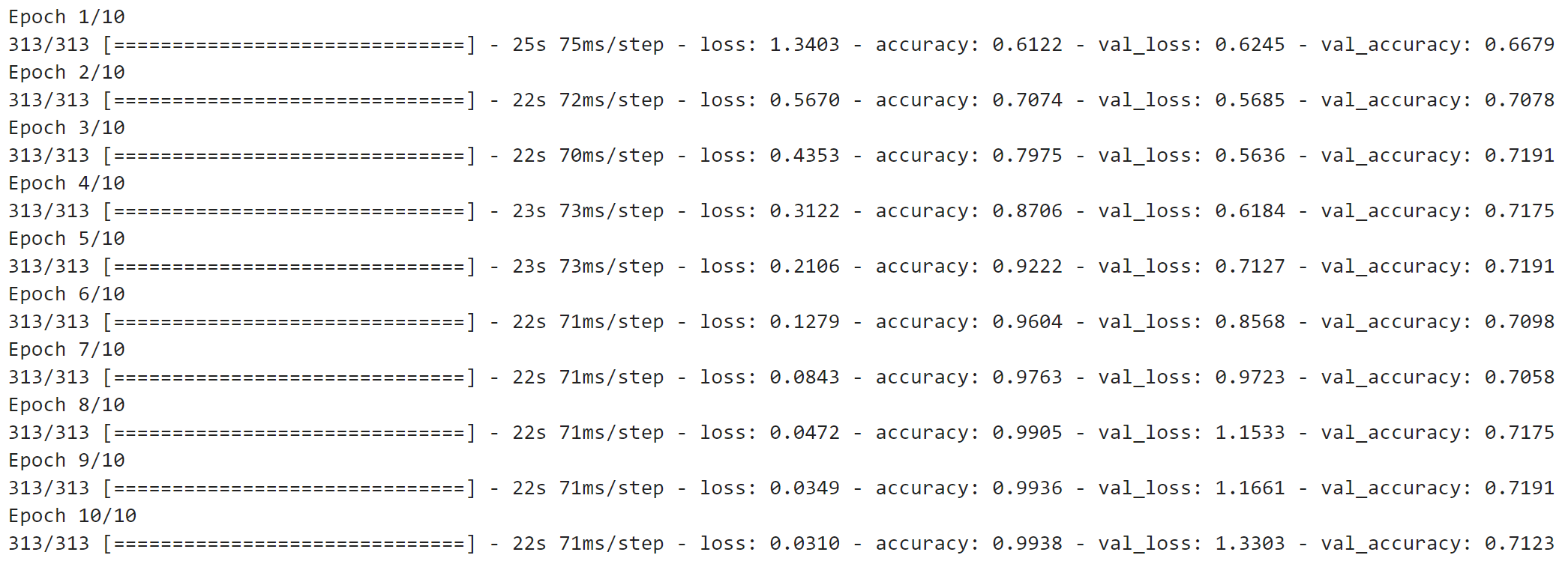
Image 13 — Model 1 training log (image by author)
Even a simple convolutional model outperforms a model with only fully-connected layers. Does doubling the number of filters make a difference?
model_2 = tf.keras.Sequential([
    tf.keras.layers.Conv2D(filters=32, kernel_size=(3, 3), input_shape=(224, 224, 3), activation='relu'),
    tf.keras.layers.MaxPool2D(pool_size=(2, 2), padding='same'),
    tf.keras.layers.Flatten(),
    tf.keras.layers.Dense(128, activation='relu'),
    tf.keras.layers.Dense(2, activation='softmax')
])

model_2.compile(
    loss=tf.keras.losses.categorical_crossentropy,
    optimizer=tf.keras.optimizers.Adam(),
    metrics=[tf.keras.metrics.BinaryAccuracy(name='accuracy')]
)

history_2 = model_2.fit(
    train_data,
    validation_data=valid_data,
    epochs=10
)
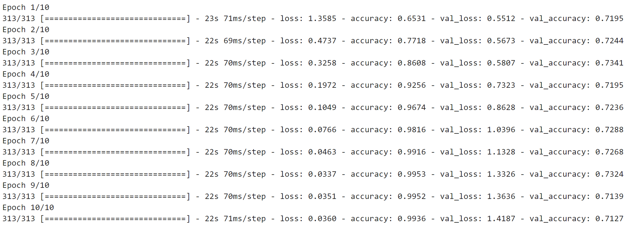
Image 14 — Model 2 training log (image by author)
Maybe, but the model doesn’t look like it’s learning. Let’s add a second Convolutional layer:
model_3 = tf.keras.Sequential([
    tf.keras.layers.Conv2D(filters=32, kernel_size=(3, 3), input_shape=(224, 224, 3), activation='relu'),
    tf.keras.layers.MaxPool2D(pool_size=(2, 2), padding='same'),
    tf.keras.layers.Conv2D(filters=32, kernel_size=(3, 3), activation='relu'),
    tf.keras.layers.MaxPool2D(pool_size=(2, 2), padding='same'),
    tf.keras.layers.Flatten(),
    tf.keras.layers.Dense(128, activation='relu'),
    tf.keras.layers.Dense(2, activation='softmax')
])

model_3.compile(
    loss=tf.keras.losses.categorical_crossentropy,
    optimizer=tf.keras.optimizers.Adam(),
    metrics=[tf.keras.metrics.BinaryAccuracy(name='accuracy')]
)

history_3 = model_3.fit(
    train_data,
    validation_data=valid_data,
    epochs=10
)
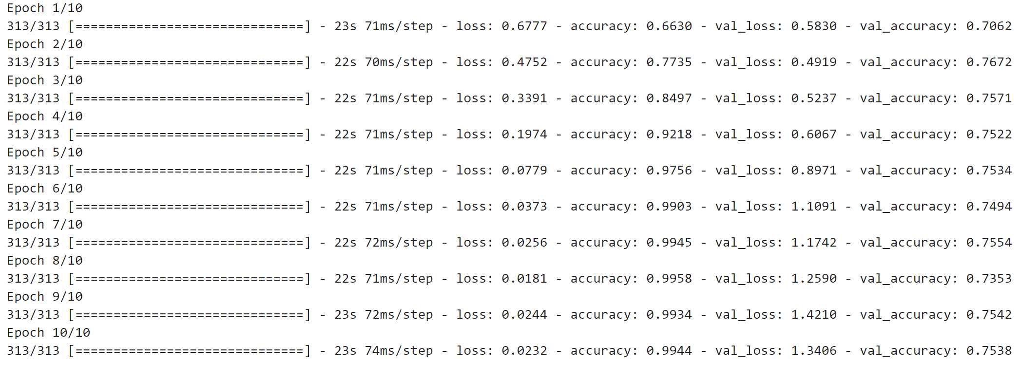
Image 15 — Model 3 training log (image by author)
That does it — 75% accuracy on the validation set. Feel free to experiment further on your own. The following section uses model_3 to make predictions on the test set.
Make Predictions on New Images
Here’s the thing — you have to apply the same preprocessing operations to the test set. I forgot this step many times, and it resulted in weird and uncertain predictions (small difference between prediction probabilities).
For that reason, we’ll declare a function that resizes a given image to 224x224 and rescales it to a 0–1 range:
def prepare_single_image(img_path: str) -> np.array:
    img = Image.open(img_path)
    img = img.resize(size=(224, 224))
    return np.array(img) / 255.0
Let’s now use it on a single image from the test set:
single_image = prepare_single_image(img_path='data/test/cat/10018.jpg')
single_prediction = model_3.predict(single_image.reshape(-1, 224, 224, 3))
single_prediction

Image 16 — Prediction probabilities for each class (image by author)
The model is almost 100% certain this is a cat image (0 = cat, 1 = dog). You can use the argmax() function to get the index where the value of an array is the highest. It returns 0, meaning the model thinks it’s a cat.
Let’s make predictions for an entire folder of images. There are smarter ways to approach this, but this method is deliberately explicit. We iterate over the folder and make predictions for a single image, and then keep track of how many images were classified correctly:
num_total_cat, num_correct_cat = 0, 0
num_total_dog, num_correct_dog = 0, 0

for img_path in pathlib.Path.cwd().joinpath('data/test/cat').iterdir():
    try:
        img = prepare_single_image(img_path=str(img_path))
        pred = model_3.predict(tf.expand_dims(img, axis=0))
        pred = pred.argmax()
        num_total_cat += 1
        if pred == 0:
            num_correct_cat += 1
    except Exception as e:
        continue

for img_path in pathlib.Path.cwd().joinpath('data/test/dog').iterdir():
    try:
        img = prepare_single_image(img_path=str(img_path))
        pred = model_3.predict(tf.expand_dims(img, axis=0))
        pred = pred.argmax()
        num_total_dog += 1
        if pred == 1:
            num_correct_dog += 1
    except Exception as e:
        continue
Here are the results for cats:
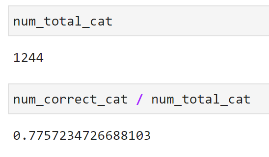
Image 17 — Model accuracy for cats (image by author)
And here are for dogs:
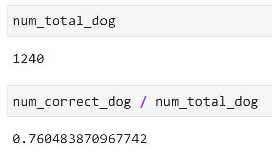
Image 18 — Model accuracy for dogs (image by author)
Overall, we have a much more accurate model than when we were only using Dense layers. This is just the tip of the iceberg, as we haven’t explored data augmentation and transfer learning yet.
You wouldn’t believe how much these will increase the accuracy.
Stay connected
- Sign up for my newsletter
- Subscribe on YouTube
- Connect on LinkedIn