TensorFlow for Computer Vision — Does a More Complex Architecture Guarantee a Better Model?

Your model architecture is probably fine. It’s the data quality that sucks.

You saw in the previous article how to train a basic image classifier with convolutional networks. We got around 75% accuracy without breaking a sweat — only by using two convolutional and two pooling layers, followed by a fully-connected layer.

Is that the best we can do? Is it worth it to add more layers? When does the model become too complex, and what happens then? These are the questions you’ll find answers to in today’s article. We’ll add multiple convolution blocks to see how much can our dogs vs. cats dataset handle.

Don’t feel like reading? Watch my video instead:

You can download the source code on GitHub.

Dataset Used and Data Preprocessing

We’ll use the Dogs vs. Cats dataset from Kaggle. It’s licensed under the Creative Commons License, which means you can use it for free:

The dataset is fairly large — 25,000 images distributed evenly between classes (12,500 dog images and 12,500 cat images). It should be big enough to train a decent image classifier. The only problem is — it’s not structured for deep learning out of the box. You can follow my previous article to create a proper directory structure, and split it into train, test, and validation sets:

TensorFlow for Computer Vision — Top 3 Prerequisites for Deep Learning Projects

You should also delete the train/cat/666.jpg and train/dog/11702.jpg images as they’re corrupted, and your model will fail to train with them.

Let’s see how to load in the images with TensorFlow next.

How to Load Image Data with TensorFlow

The models you’ll see today will have more layers than the ones in the previous articles. For readability sake, we’ll import individual classes from TensorFlow. Make sure to have a system with a GPU if you’re following along, or at least use Google Colab.

Let’s get the library imports out of the way:

import os
os.environ['TF_CPP_MIN_LOG_LEVEL'] = '2'

import warnings
warnings.filterwarnings('ignore')

import tensorflow as tf
from tensorflow.keras import Sequential
from tensorflow.keras.layers import Conv2D, MaxPool2D, Flatten, Dense, Dropout
from tensorflow.keras.preprocessing.image import ImageDataGenerator
from tensorflow.keras.losses import categorical_crossentropy
from tensorflow.keras.optimizers import Adam
from tensorflow.keras.metrics import BinaryAccuracy

tf.random.set_seed(42)
physical_devices = tf.config.list_physical_devices('GPU')
try:
    tf.config.experimental.set_memory_growth(physical_devices[0], True)
except:
    pass

It’s a lot, but the models will look extra clean because of it.

We’ll now load in the image data as we normally would — with the ImageDataGenerator class. We’ll convert the image matrices to a 0–1 range, and resize all images to 224x224 with three color channels. For memory concerns, we’ll lower the batch size to 32:

train_datagen = ImageDataGenerator(rescale=1/255.0)
valid_datagen = ImageDataGenerator(rescale=1/255.0)

train_data = train_datagen.flow_from_directory(
    directory='data/train/',
    target_size=(224, 224),
    class_mode='categorical',
    batch_size=32,
    shuffle=True,
    seed=42
)

valid_data = valid_datagen.flow_from_directory(
    directory='data/validation/',
    target_size=(224, 224),
    class_mode='categorical',
    batch_size=32,
    seed=42
)

Here’s the output you should see:

That’s all we need — let’s crack the first model!

Does Adding Layers to a TensorFlow Model Make Any Difference?

Writing convolutional models from scratch is always a tricky task. Grid searching the optimal architecture isn’t feasible, as convolutional models take a long time to train, and there are too many moving parts to check. In reality, you’re far more likely to use transfer learning. That’s a topic we’ll explore in the near future.

Today, it’s all about understanding why going big with the model architecture isn’t worth it. We got 75% accuracy with somewhat of a simple model, so that’s the baseline we have to outperform:

TensorFlow for Computer Vision — How to Train Image Classifiers with Convolutional Neural Networks

Model 1 — Two convolutional blocks

We’ll declare the first model to somewhat resemble the VGG architecture — two convolutional layers followed by a pooling layer. We won’t go crazy with the number of filters — 32 for the first and 64 for the second block.

As for the loss and optimizer, we’ll stick with the basics — categorical cross-entropy and Adam. The classes in the dataset are perfectly balanced, which means we can get around with only tracking the accuracy:

model_1 = tf.keras.Sequential([
    Conv2D(filters=32, kernel_size=(3, 3), input_shape=(224, 224, 3), activation='relu'),
    Conv2D(filters=32, kernel_size=(3, 3), activation='relu'),
    MaxPool2D(pool_size=(2, 2), padding='same'),
    
    Conv2D(filters=64, kernel_size=(3, 3), activation='relu'),
    Conv2D(filters=64, kernel_size=(3, 3), activation='relu'),
    MaxPool2D(pool_size=(2, 2), padding='same'),
    
    Flatten(),
    Dense(units=128, activation='relu'),
    Dense(units=2, activation='softmax')
])


model_1.compile(
    loss=categorical_crossentropy,
    optimizer=Adam(),
    metrics=[BinaryAccuracy(name='accuracy')]
)
model_1_history = model_1.fit(
    train_data,
    validation_data=valid_data,
    epochs=10
)

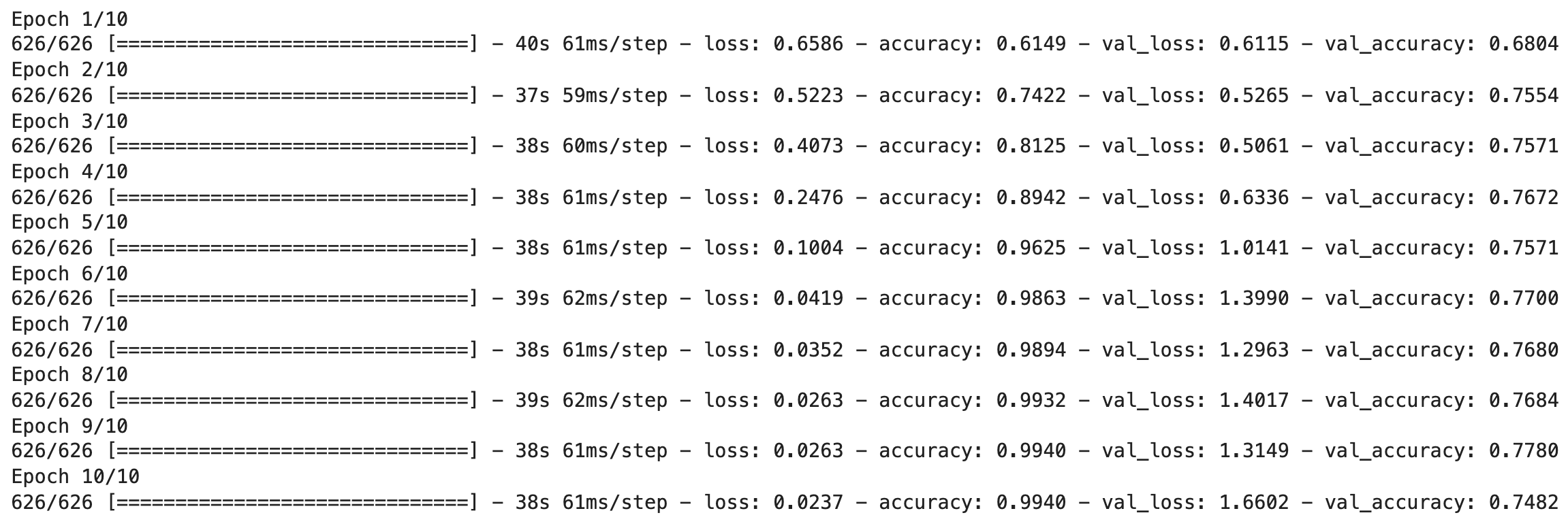
Here are the training results after 10 epochs:

It looks like we didn’t outperform the baseline, as the validation accuracy is still around 75%. What will happen if we add yet another convolutional block?

Model 2 — Three convolutional blocks

We’ll keep the model architecture identical, the only difference being an additional convolutional block with 128 filters:

model_2 = Sequential([
    Conv2D(filters=32, kernel_size=(3, 3), input_shape=(224, 224, 3), activation='relu'),
    Conv2D(filters=32, kernel_size=(3, 3), activation='relu'),
    MaxPool2D(pool_size=(2, 2), padding='same'),
    
    Conv2D(filters=64, kernel_size=(3, 3), activation='relu'),
    Conv2D(filters=64, kernel_size=(3, 3), activation='relu'),
    MaxPool2D(pool_size=(2, 2), padding='same'),
    
    Conv2D(filters=128, kernel_size=(3, 3), activation='relu'),
    Conv2D(filters=128, kernel_size=(3, 3), activation='relu'),
    MaxPool2D(pool_size=(2, 2), padding='same'),
    
    Flatten(),
    Dense(units=128, activation='relu'),
    Dense(units=2, activation='softmax')
])


model_2.compile(
    loss=categorical_crossentropy,
    optimizer=Adam(),
    metrics=[BinaryAccuracy(name='accuracy')]
)
model_2_history = model_2.fit(
    train_data,
    validation_data=valid_data,
    epochs=10
)

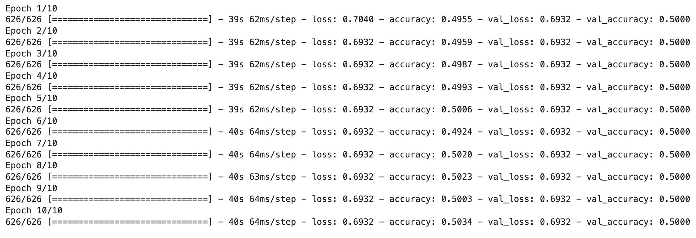
Here’s the log:

Yikes. The model is completely stuck. You could play around with the batch size and learning rate, but you likely won’t get far. The first architecture worked better on our dataset, so let’s try tweaking it a bit.

Model 3 — Two convolutional blocks with a dropout

The architecture of the third model is identical to the first one, the only difference is an additional fully-connected layer and a dropout layer. Let’s see if it makes a difference:

model_3 = tf.keras.Sequential([
    Conv2D(filters=32, kernel_size=(3, 3), input_shape=(224, 224, 3), activation='relu'),
    Conv2D(filters=32, kernel_size=(3, 3), activation='relu'),
    MaxPool2D(pool_size=(2, 2), padding='same'),
    
    Conv2D(filters=64, kernel_size=(3, 3), activation='relu'),
    Conv2D(filters=64, kernel_size=(3, 3), activation='relu'),
    MaxPool2D(pool_size=(2, 2), padding='same'),
    
    Flatten(),
    Dense(units=512, activation='relu'),
    Dropout(rate=0.3),
    Dense(units=128),
    Dense(units=2, activation='softmax')
])

model_3.compile(
    loss=categorical_crossentropy,
    optimizer=Adam(),
    metrics=[BinaryAccuracy(name='accuracy')]
)

model_3_history = model_3.fit(
    train_data,
    validation_data=valid_data,
    epochs=10
)

Here is the training log:

Horrible, we’re below 70% now!. That’s what happens when you focus on the wrong thing. The simple architecture from the previous article was completely fine. It’s the problem of data quality that limits the predictive power of your model.

Conclusion

And there you have it — proof that a more complex model architecture doesn’t necessarily result in a better-performing model. Maybe you could find an architecture that’s better suited for the dogs vs. cats dataset, but it’s likely a wild goose chase.

You should shift the focus to improving the dataset quality. Sure, there are 20K training images, but we can still add variety to it. That’s where data augmentation comes in handy, and you’ll learn all about it in the following article. After that, you’ll take your models to new heights with transfer learning, which will make hand-tuning convolutional models look like a dumb thing to do.

Stay tuned for the upcoming articles, as both are a must-know for a modern-day data scientist.

Stay connected

• Sign up for my newsletter
• Subscribe on YouTube
• Connect on LinkedIn