
Image classification without convolutions? Here’s why it’s a bad idea
Artificial neural networks aren’t designed for image classification. But how terrible can they be? That’s what we’ll find out today. We’ll train an image classification model on 20,000 images using only Dense layers. So no convolutions and other fancy stuff, we’ll save them for upcoming articles.
It goes without saying, but you really shouldn’t use vanilla Artificial neural networks to classify images. Images are two-dimensional, and you’ll lose the patterns which make images recognizable by flattening them. Still, it’s fun and doable, and will give you insight into everything wrong with this approach.
Don’t feel like reading? Watch my video instead:
You can download the source code on GitHub.
Dataset used and data preparation
We’ll use the Dogs vs. Cats dataset from Kaggle. It’s licensed under the Creative Commons License, which means you can use it for free:
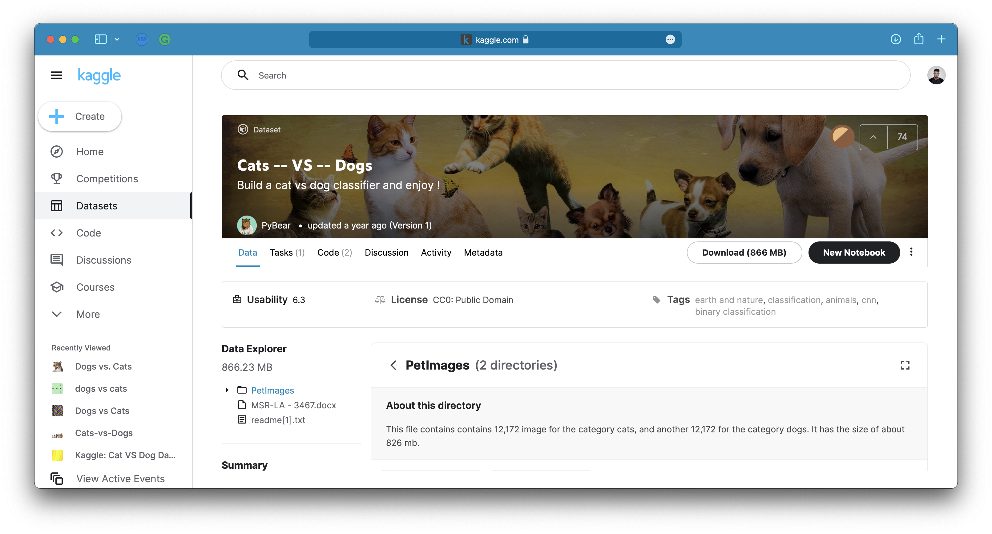
Image 1 — Dogs vs. Cats dataset (image by author)
The dataset is fairly large — 25,000 images distributed evenly between classes (12,500 dog images and 12,500 cat images). It should be big enough to train a decent image classifier, but not with ANNs.
The only problem is — it’s not structured properly for deep learning out of the box. You can follow my previous article to create a proper directory structure, and split it into train, test, and validation sets:
TensorFlow for Computer Vision — Top 3 Prerequisites for Deep Learning Projects
Downsize, grayscale, and flatten images
Let’s get the library imports out of the way. We’ll need quite a few of them, so make sure to have Numpy, Pandas, TensorFlow, PIL, and Scikit-Learn installed:
import os
import pathlib
import pickle
import numpy as np
import pandas as pd
import tensorflow as tf
from PIL import Image, ImageOps
from IPython.display import display
from sklearn.utils import shuffle
import matplotlib.pyplot as plt
from matplotlib import rcParams
import warnings

os.environ['TF_CPP_MIN_LOG_LEVEL'] = '2'
warnings.filterwarnings('ignore')
rcParams['figure.figsize'] = (18, 8)
rcParams['axes.spines.top'] = False
rcParams['axes.spines.right'] = False
You can’t pass an image directly to a Dense layer. A single image is 3-dimensional — height, width, color channels — and a Dense layer expects a 1-dimensional input.
Let’s take a look at an example. The following code loads and displays a cat image from the training set:
src_img = Image.open('data/train/cat/1.jpg')
display(src_img)
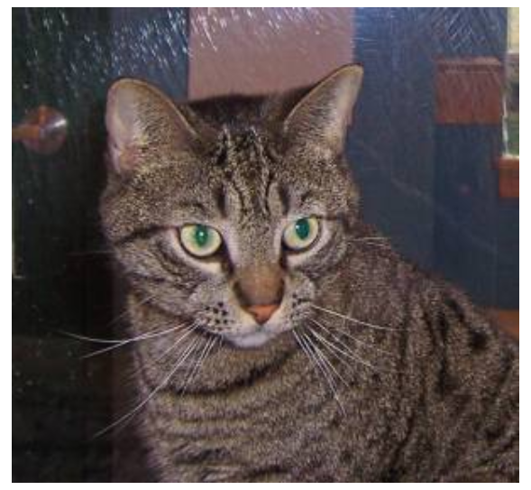
Image 2 — Example cat image (image by author)
The image is 281 pixels wide, 300 pixels tall, and has three color channels (np.array(src_img).shape ). In total, it has 252,900 pixels, which translates into 252,900 features when flattened. It’s a lot, so let’s save some resources where possible.
You should grayscale your image dataset if it makes sense. If you can classify images that aren’t displayed in color, so should the neural network. You can use the following code snippet to convert the image to grayscale:
gray_img = ImageOps.grayscale(src_img)
display(gray_img)
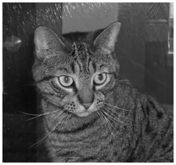
Image 3 — Grayscale cat image (image by author)
It’s still a cat, obviously, so the color doesn’t play a big role in this dataset. The grayscaled image is 281 pixels wide and 300 pixels tall, but has a single color channel. It means we went from 252,900 to 84,300 pixels. Still a lot, but definitely a step in the right direction.
As discussed in the previous article, the images in the dataset don’t have identical sizes. It’s a problem for a neural network model, as it expects the same number of input features every time. We can resize every image to the same width and height. This is where we introduce downsizing, to reduce the number of input features further.
The following code snippet resizes our image so it’s both 96 pixels wide and tall:
gray_resized_img = gray_img.resize(size=(96, 96))
display(gray_resized_img)
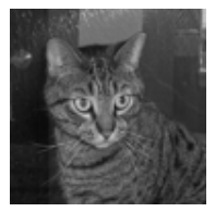
Image 4 — Resized cat image (image by author)
The image is somewhat small and blurry, sure, but it’s still a cat. We’re down to 9,216 features, in case you’re keeping track. We’ve reduced the number of features by a factor of 27, which is a big deal.
As the last step, we need to flatten the image. You can use the ravel() function from Numpy to do so:
np.ravel(gray_resized_img)

Image 5 — Flattened cat image (image by author)
That’s how a computer sees a cat — it’s just an array of 9216 pixels, ranging from 0 to 255. Here’s the problem — a neural network prefers a range between 0 and 1. Dividing the entire array by 255.0 does the trick:
img_final = np.ravel(gray_resized_img) / 255.0
img_final

Image 6 — Flattened and scaled cat image (image by author)
As the last step, we’ll write a process_image() function that applies all the above transformations to a single image:
def process_image(img_path: str) -> np.array:
    img = Image.open(img_path)
    img = ImageOps.grayscale(img)
    img = img.resize(size=(96, 96))
    img = np.ravel(img) / 255.0
    return img
Let’s test it on a random dog image, and then reverse the last step to represent the image visually:
tst_img = process_image(img_path='data/validation/dog/10012.jpg')
Image.fromarray(np.uint8(tst_img * 255).reshape((96, 96)))
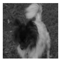
Image 7 — Transformed dog image (image by author)
And that’s it — the function works as advertised. Let’s apply it to the entire dataset next.
Convert image to tabular data for deep learning
We’ll write yet another function —process_folder()— which iterates over a given folder and uses the process_image() function on any JPG file. It then combines all images into a single Pandas DataFrame and adds a class as an additional column (cat or dog):
def process_folder(folder: pathlib.PosixPath) -> pd.DataFrame:
    # We'll store the images here
    processed = []

    # For every image in the directory
    for img in folder.iterdir():
        # Ensure JPG
        if img.suffix == '.jpg':
            # Two images failed for whatever reason, so let's just ignore them
            try:
                processed.append(process_image(img_path=str(img)))
            except Exception as _:
                continue

    # Convert to pd.DataFrame
    processed = pd.DataFrame(processed)
    # Add a class column - dog or a cat
    processed['class'] = folder.parts[-1]

    return processed
Let’s apply it to train, test, and validation folders. You’ll need to call it twice per folder, once for cats and once for dogs, and then concatenate the sets. We’ll also dump the datasets into a pickle file:
# Training set
train_cat = process_folder(folder=pathlib.Path.cwd().joinpath('data/train/cat'))
train_dog = process_folder(folder=pathlib.Path.cwd().joinpath('data/train/dog'))
train_set = pd.concat([train_cat, train_dog], axis=0)

with open('train_set.pkl', 'wb') as f:
    pickle.dump(train_set, f)

# Test set
test_cat = process_folder(folder=pathlib.Path.cwd().joinpath('data/test/cat'))
test_dog = process_folder(folder=pathlib.Path.cwd().joinpath('data/test/dog'))
test_set = pd.concat([test_cat, test_dog], axis=0)

with open('test_set.pkl', 'wb') as f:
    pickle.dump(test_set, f)

# Validation set
valid_cat = process_folder(folder=pathlib.Path.cwd().joinpath('data/validation/cat'))
valid_dog = process_folder(folder=pathlib.Path.cwd().joinpath('data/validation/dog'))
valid_set = pd.concat([valid_cat, valid_dog], axis=0)

with open('valid_set.pkl', 'wb') as f:
    pickle.dump(valid_set, f)
Here’s how the train_set looks like:
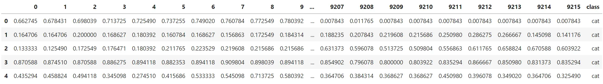
Image 8 — Head of the training set (image by author)
The datasets contain all cat images followed by all dog images. That’s not ideal for training and validation sets, as the neural network will see them in that order. You can use the shuffle function from Scikit-Learn to randomize the ordering:
train_set = shuffle(train_set).reset_index(drop=True)
valid_set = shuffle(valid_set).reset_index(drop=True)
Here’s how it looks like now:
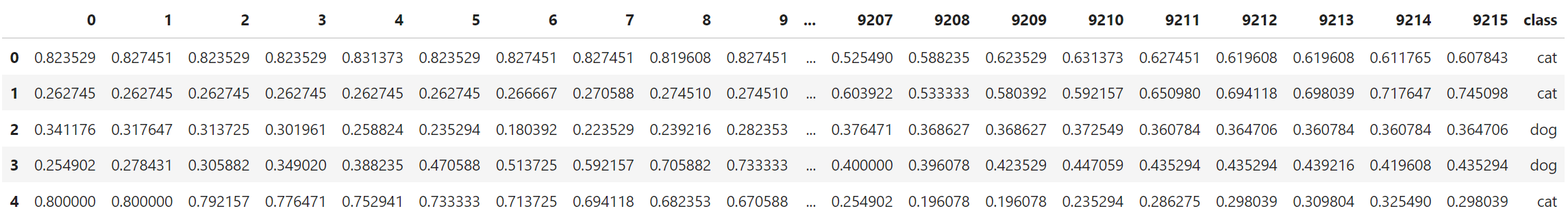
Image 9 — Head of the shuffled training set (image by author)
Almost there. The next step is to separate the features from the target, just as you normally would do on any tabular dataset. We’ll do the split for all three subsets:
X_train = train_set.drop('class', axis=1)
y_train = train_set['class']

X_valid = valid_set.drop('class', axis=1)
y_valid = valid_set['class']

X_test = test_set.drop('class', axis=1)
y_test = test_set['class']
And finally, you must factorize the target variable. There are two distinct classes (cat and dog), so the target variable for each instance should contain two elements. For example, here’s what the factorize() function does when applied to y_train:
y_train.factorize()
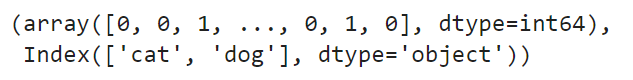
Image 10 — Factorize function applied to y_train (image by author)
The labels got converted into integers — 0 for cats and 1 for dogs. You can use the to_categorical() function from TensorFlow and pass in the array of factorized integer representations, alongside the number of distinct classes (2):
y_train = tf.keras.utils.to_categorical(y_train.factorize()[0], num_classes=2)
y_valid = tf.keras.utils.to_categorical(y_valid.factorize()[0], num_classes=2)
y_test = tf.keras.utils.to_categorical(y_test.factorize()[0], num_classes=2)
As a result, y_train now looks like this:
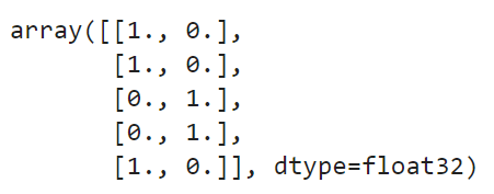
Image 11 — Target variable in a categorical format (image by author)
Think of it in terms of probability — the first image has a 100% chance of being a cat, and a 0% chance of being a dog. These are true labels, so the probability can be either 0 or 1.
We now finally have everything needed to train a neural network model.
Train an image classification model with an Artificial neural network (ANN)
I’ve chosen the number of layers and the number of nodes per layer randomly. You are welcome to tune the network however you want. You shouldn’t change the following:
- Output layer— It needs two nodes as we have two distinct classes. We can’t use the sigmoid activation function anymore, so opt for softmax.
- Loss function— Binary cross entropy won’t cut it. Go with the categorical cross entropy.
Everything else is completely up to you:
tf.random.set_seed(42)

model = tf.keras.Sequential([
    tf.keras.layers.Dense(2048, activation='relu'),
    tf.keras.layers.Dense(1024, activation='relu'),
    tf.keras.layers.Dense(1024, activation='relu'),
    tf.keras.layers.Dense(128, activation='relu'),
    tf.keras.layers.Dense(2, activation='softmax')
])

model.compile(
    loss=tf.keras.losses.categorical_crossentropy,
    optimizer=tf.keras.optimizers.Adam(),
    metrics=[tf.keras.metrics.BinaryAccuracy(name='accuracy')]
)

history = model.fit(
    X_train,
    y_train,
    epochs=100,
    batch_size=128,
    validation_data=(X_valid, y_valid)
)
Here are the results I got after 100 epochs:
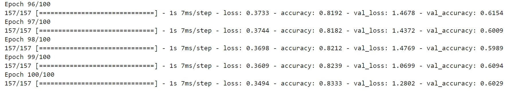
Image 12 — ANN results after 100 epochs (image by author)
A 60% accuracy is just a tad better from guessing, but nothing to write home about. Still, let’s inspect what happened to the metrics during the training.
The following code snippet plots training loss vs. validation loss for each of the 100 epochs:
plt.plot(np.arange(1, 101), history.history['loss'], label='Training Loss')
plt.plot(np.arange(1, 101), history.history['val_loss'], label='Validation Loss')
plt.title('Training vs. Validation Loss', size=20)
plt.xlabel('Epoch', size=14)
plt.legend();
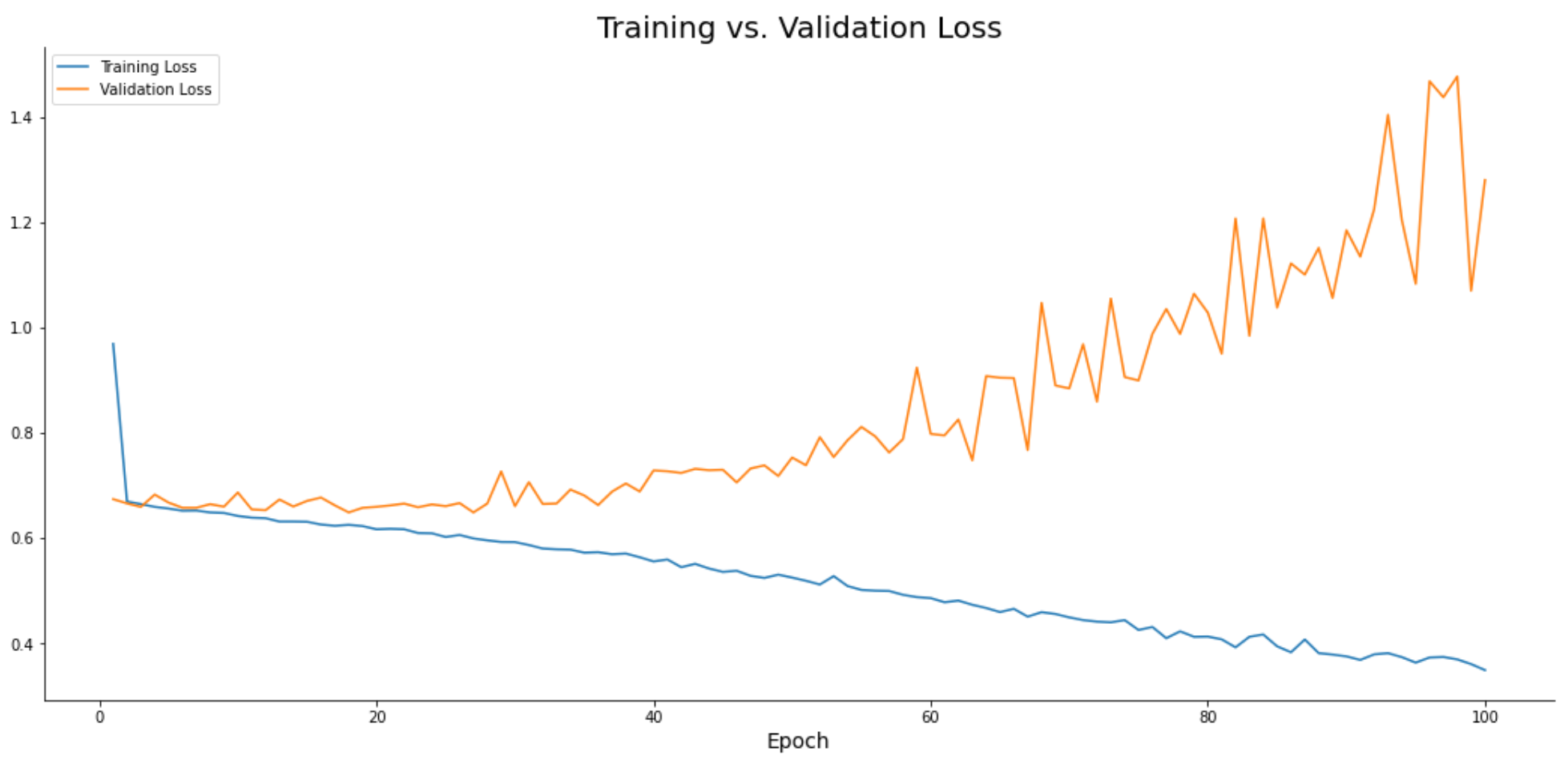
Image 13 — Training loss vs. validation loss (image by author)
The model is learning the training data well, but fails to generalize. The validation loss continues to increase as we train the model for more epochs, indicating an unstable and unusable model.
Let’s see how do the accuracies compare:
plt.plot(np.arange(1, 101), history.history['accuracy'], label='Training Accuracy')
plt.plot(np.arange(1, 101), history.history['val_accuracy'], label='Validation Accuracy')
plt.title('Training vs. Validation Accuracy', size=20)
plt.xlabel('Epoch', size=14)
plt.legend();
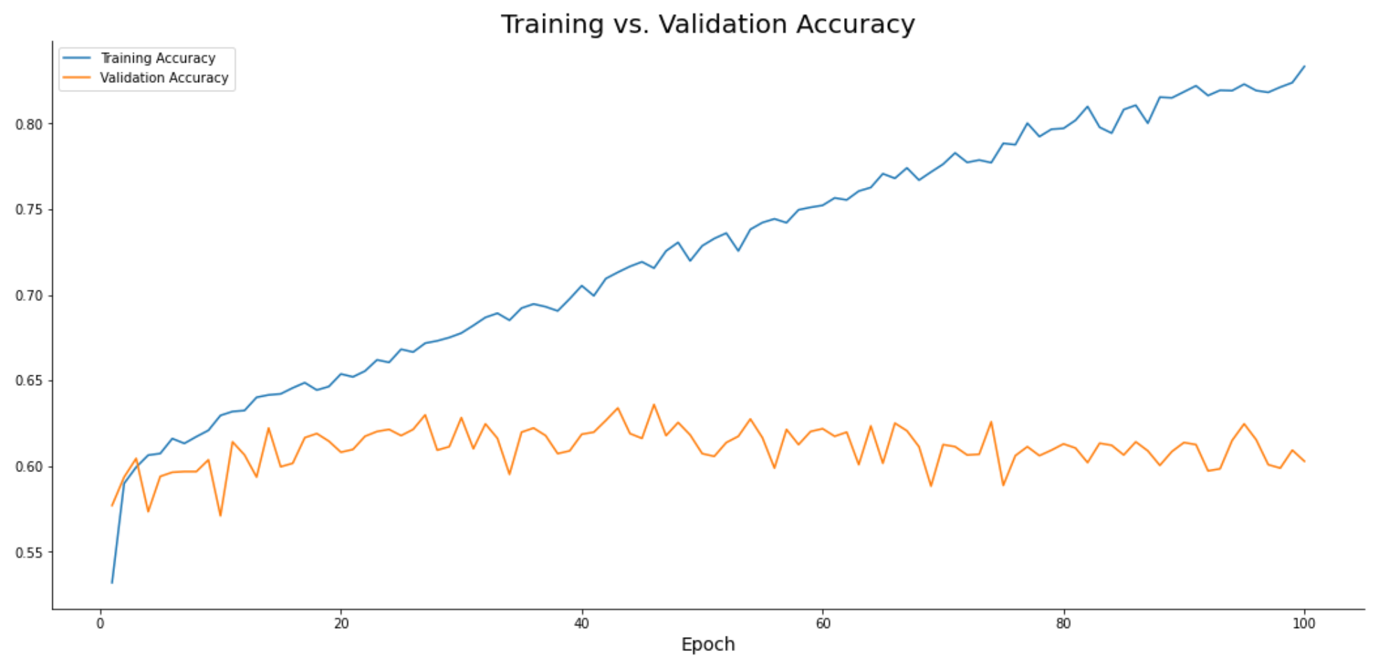
Image 14 — Training accuracy vs. validation accuracy (image by author)
Similar picture. The validation accuracy plateaus around 60%, while the model overfits on the training data.
60% accuracy for a two-class dataset with 20K training images is almost as bad as it can get. The reason is simple —Dense layers aren’t designed to capture the complexity of 2-dimensional image data. You’ll need a conolutional layer to do the job right.
Conclusion
And there you have it — how to train an image classification model with artificial neural networks, and why you shouldn’t do it. It’s like climbing a mountain in flip-flops — maybe you can do it, but it’s better not to.
You learn how the convolutional neural networks work in the following article, and you’ll see the improvement they bring. I’ll release that article on Friday, so stay tuned.
Stay connected
- Sign up for my newsletter
- Subscribe on YouTube
- Connect on LinkedIn