Newcomers to data science - including myself a couple of years ago - suffer from the same problem. They use Python for everything, from gathering to storing and manipulating data. Sure, modern programming languages can handle everything, but is it really the best strategy? It’s not, and you’ll see why today.
SQL isn’t the sexiest language, mostly because it’s been around the block for what seems like forever. Everyone and their mothers claim their know SQL, but just because you can fetch all columns from a table doesn’t mean you’re a proficient user.
Today we’ll take a look at the following scenario: A company stores tens of million rows on a local Postgres database. They want to know how much faster aggregating data on a database is when compared to fetching all data with Python and doing aggregations there.
Don’t feel like reading? I’ve covered the same topic in a video format:
Create a Synthetic Dataset with Python
First things first, we’ll have to create a dataset. You’ll need Numpy, Pandas, and Psycopg2 installed (for Postgres connection). Here are the imports:
import random
import string
import warnings
import psycopg2
import numpy as np
import pandas as pd
from datetime import datetime

np.random.seed = 42
warnings.filterwarnings('ignore')
As for the data, we’ll create a synthetic dataset ranging from 1920 to 2020, and it’ll imitate the company’s sales across different departments. Here are the functions we’ll need:
def get_department() -> str:
    x = np.random.rand()
    if x < 0.2: return 'A'
    elif 0.2 <= x < 0.4: return 'B'
    elif 0.4 <= x < 0.6: return 'C'
    elif 0.6 <= x < 0.8: return 'D'
    else: return 'E'

def gen_random_string(length: int = 32) -> str:
    return ''.join(random.choices(
        string.ascii_uppercase + string.digits, k=length)
    )

date_range = pd.date_range(
    start=datetime(1920, 1, 1),
    end=datetime(2020, 1, 1),
    freq='120s'
)

df_size = len(date_range)
We can use them to create the dataset:
df = pd.DataFrame({
    'datetime': date_range,
    'department': [get_department() for x in range(df_size)],
    'items_sold': [np.random.randint(low=0, high=100) for x in range(df_size)],
    'string': [gen_random_string() for x in range(df_size)],
})
Here’s what it looks like:
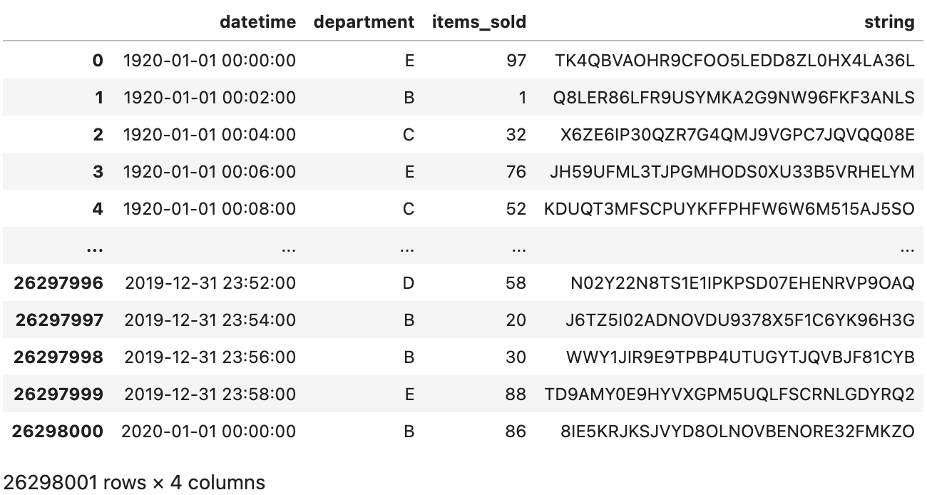
Image 1 - Synthetic 26M row dataset (image by author)
Over 26M rows spread over four columns. It’s not the most realistic-looking table, I’ll give you that, but it’s still a decent amount of data. Let’s dump it into a CSV file:
df.to_csv('df.csv', index=False)
It takes 1,52 GB of space on a disk, which isn’t considered big by today’s standards.
Load the Dataset into Postgres Database
The next step is to create a table in Postgres and load the CSV file. Onto the table first - it’ll have a primary key column in addition to the other four. I like adding prefixes to column names, but you don’t have to:
CREATE TABLE department_sales(
	dsl_id SERIAL PRIMARY KEY,
	dsl_datetime TIMESTAMP,
	dsl_department CHAR(1),
	dsl_items_sold SMALLINT,
	dsl_string VARCHAR(32)
);
Issue the following command to copy the contents of the CSV file into our Postgres table - just remember to change the path:
COPY department_sales(dsl_datetime, dsl_department, dsl_items_sold, dsl_string)
FROM '/Users/dradecic/Desktop/df.csv'
DELIMITER ','
CSV HEADER;
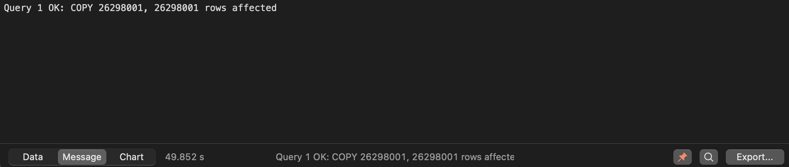
Image 2 - Dataset copying results (image by author)
And there it is - over 26M rows loaded in just under 50 seconds. Let’s run a SELECT statement to see if everything looks alright:
SELECT * FROM department_sales;
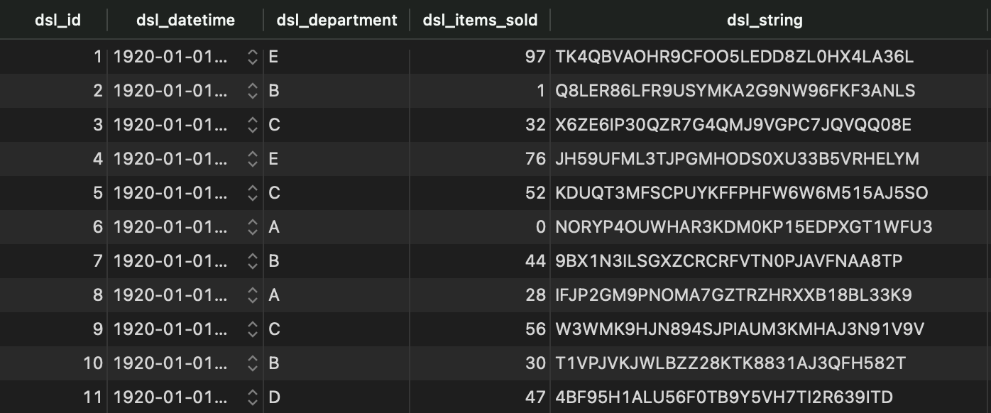
Image 3 - Synthetic dataset in Postgres database (image by author)
It does - so let’s load the data with Python next.
Option #1 - Load the Entire Table with Python
Use the connect() method from Psycopg2 to establish a database connection through Python:
conn = psycopg2.connect(
    user='<username>',
    password='<password>',
    host='127.0.0.1',
    port=5432,
    database='<db>'
)
We can now issue the same SELECT statement as we did earlier through the DBMS:
%%time

df_department_sales = pd.read_sql("SELECT * FROM department_sales", conn)

Image 4 - Time required to load 26M rows from Postgres to Python (image by author)
It took 75 seconds to fetch 26M rows, which isn’t too bad. That’s mostly because the database isn’t in the cloud. Still, 75 seconds can be a long time to wait if speed is the key.
Let’s aggregate the data now. We’ll group it by the department and calculate the sum of items sold:
%%time

df_pd_sales_by_department = (
    df_department_sales
        .groupby('dsl_department')
        .sum()
        .reset_index()
)[['dsl_department', 'dsl_items_sold']]

df_pd_sales_by_department
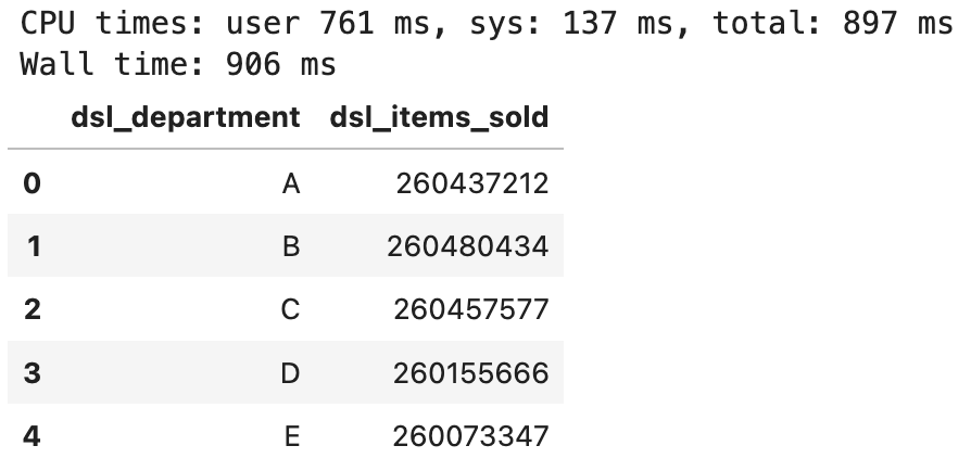
Image 5 - Aggregated view of items sold per department (image by author)
Under a second, which is expected. I’m running the notebook on M1 Pro MacBook Pro 16" which is blazing fast, so the results don’t surprise me.
We’ll make another aggregation - this time we’ll group by year and calculate the total number of items sold per year:
%%time

df_pd_sales_by_year = (
    df_department_sales
        .groupby(df_department_sales['dsl_datetime'].dt.year)
        .sum()
        .reset_index()
)[['dsl_datetime', 'dsl_items_sold']]

df_pd_sales_by_year
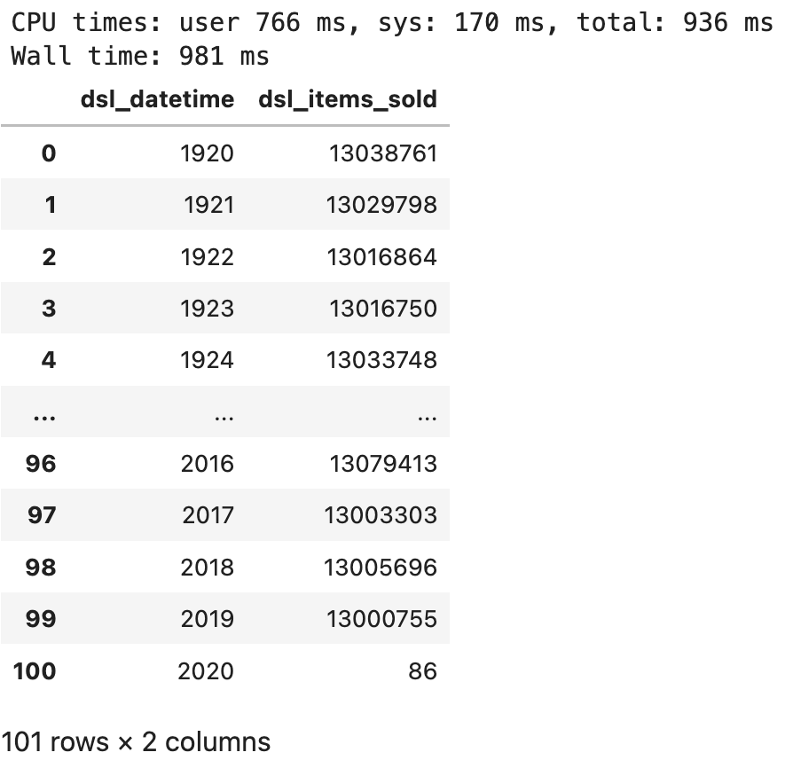
Image 6 - Aggregated view of items sold per year (image by author)
Almost identical results. Overall, we can round the runtime to 77 seconds. Let’s examine the performance of the database next.
Option #2 - Load the Prepared Views with Python
The best practice when dealing with large amounts of data is to create views in a database that contain the results of your queries. For that reason, we’ll have to issue a couple of SQL statements first.
Create Views Based on Data Aggregations in Postgres Database
This one aggregates the number of items sold by department:
CREATE OR REPLACE VIEW v_sales_by_department AS (
	SELECT
		dsl_department AS "Department",
		SUM(dsl_items_sold) AS "Total items sold"
	FROM department_sales
	GROUP BY dsl_department
	ORDER BY 2 DESC
);
Let’s see what it looks like:
SELECT * FROM v_sales_by_department;
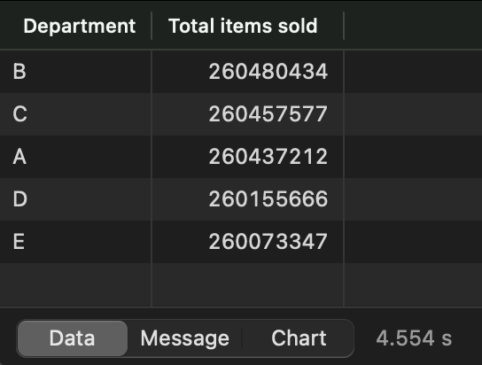
Image 7 - Items sold per department view (image by author)
It’s identical to our first aggregation operation in Python, as expected. While here, let’s create a second view that aggregates the sales amounts by year:
CREATE OR REPLACE VIEW v_sales_by_year AS (
	SELECT
		EXTRACT(YEAR FROM dsl_datetime) AS "Year",
		SUM(dsl_items_sold) AS "Total items sold"
	FROM department_sales
	GROUP BY "Year"
);
Just a quick check:
SELECT * FROM v_sales_by_year;
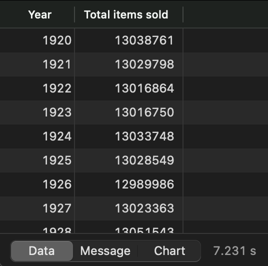
Image 8 - Items sold per year view (image by author)
Everything looks good, so let’s fetch the data from these views with Python.
Load the Data from Views with Python
First, let’s get the data for sales by department:
%%time

df_sales_by_department = pd.read_sql("SELECT * FROM v_sales_by_department", conn)
df_sales_by_department
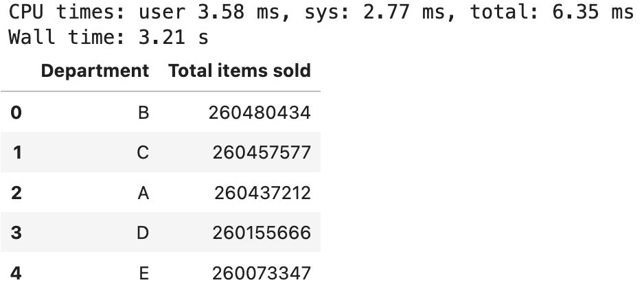
Image 9 - Fetching v_sales_by_department from Postgres database (image by author)
Three. Freaking. Seconds. Let’s do the same for the sales by year view:
%%time

df_sales_by_year = pd.read_sql("SELECT * FROM v_sales_by_year", conn)
df_sales_by_year
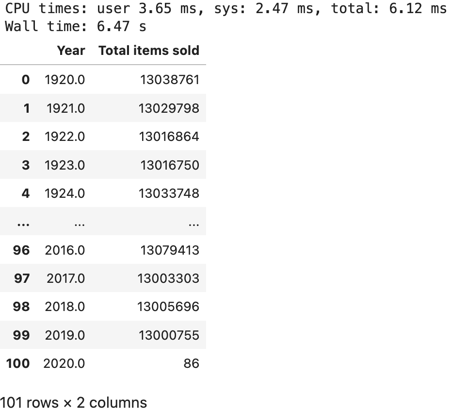
Image 10 - Fetching v_sales_by_year from Postgres database (image by author)
A bit longer, but still within reason. We can round the runtime to 10 seconds for both.
The Verdict
And there you have it - it’s almost 8 times faster to load prepared views with Python than to fetch the entire tables and do the aggregations on the fly. Keep in mind - it’s 8 times faster for local Postgres database installation, and the results would be nowhere near this if we migrated the database to the cloud.
Let me know if that’s a comparison you want to see, and I’ll be happy to cover it in a follow-up article.
The moral of the story - always leverage the database for heavy lifting. These systems are designed to work with data. Python can do it, sure, but it’s not its primary use case.
Learn More
- 5 Best Books to Learn Data Science in 2022
- How to Install Apache Airflow Locally
- Google Colab vs. RTX3060Ti for Deep Learning
Stay connected
- Hire me as a technical writer
- Subscribe on YouTube
- Connect on LinkedIn