Simple Regression with Artificial Neural Networks (ANN) in PyTorch
When it comes to supervised learning powered by neural networks, you can either go for regression or classification. This article will focus on the prior, but stay tuned for an introduction article to classification.
After reading, you’ll know how to make a synthetic dataset in Python, how to train a neural network model in PyTorch for regression, how to visualize model performance, and how large of an impact network architecture has on the predictive performance.
This is by no means a comprehensive guide - we’ll only scratch the surface. But it’s the surface that needs to be scratched for the more complex topics coming up soon.
Table of contents:
How to Create a Regression Dataset in PyTorch
Okay, so why a synthetic dataset? After all, there are so many real datasets to choose from. The answer is simple - it allows you to get a visual insight into how a neural network works.
We’ll construct a dataset that has only one feature, which means the inputs and the target variable can be plotted on a single 2-dimensional chart. This allows you to visualize the predicted values and inspect if your network “gets it”.
On the opposite side, you can only rely on mathematics with more complex and higher-dimensional data.
Anyhow, here are the library imports you’ll need today. You have all of them installed if you’ve gone through the PyTorch installation article:
import numpy as np

import torch
import torch.nn as nn
import torch.nn.functional as F

import matplotlib.pyplot as plt
import matplotlib_inline
matplotlib_inline.backend_inline.set_matplotlib_formats("svg")
The dataset will have 100 linearly spaced points in a range from -5 to +5. The torch.linspace() function is your friend here, but you’ll have to reshape the data to a row-vector format. Think of it as a single column of a DataFrame.
Regarding the target variable, it’s the input feature squared with an addition of some noise from a standard normal distribution. It needs to have the same shape as x:
# Number of data points
n = 100

# X-axis: N linearly spaced numbers between -5 and +5
x = torch.linspace(-5, 5, n).reshape(n, -1)

# Y-axis: current x squared with some random noise
y = torch.tensor([num**2 + torch.randn(1).item() for num in x]).reshape(n, -1)
Let’s print the first couple of entries from both to see what we’re dealing with:
x[:5], y[:5]
Your x tensor will be identical to mine - but y will be different due to randomization in the noise:
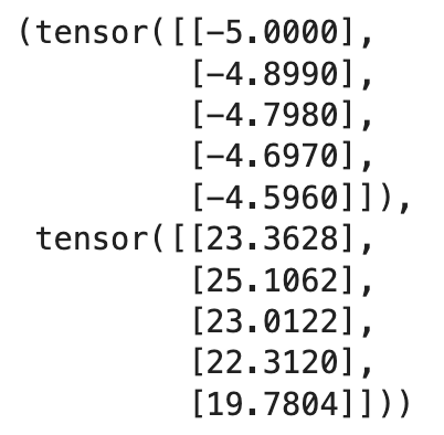
Image 1 - Contents of the X and Y tensors (Image by author)
Further, let’s explore them visually with Matplotlib:
# Visualize the data
plt.figure(figsize=(10, 7))

plt.scatter(x, y, c="#000")
plt.show()
We get a nice parabola shape:
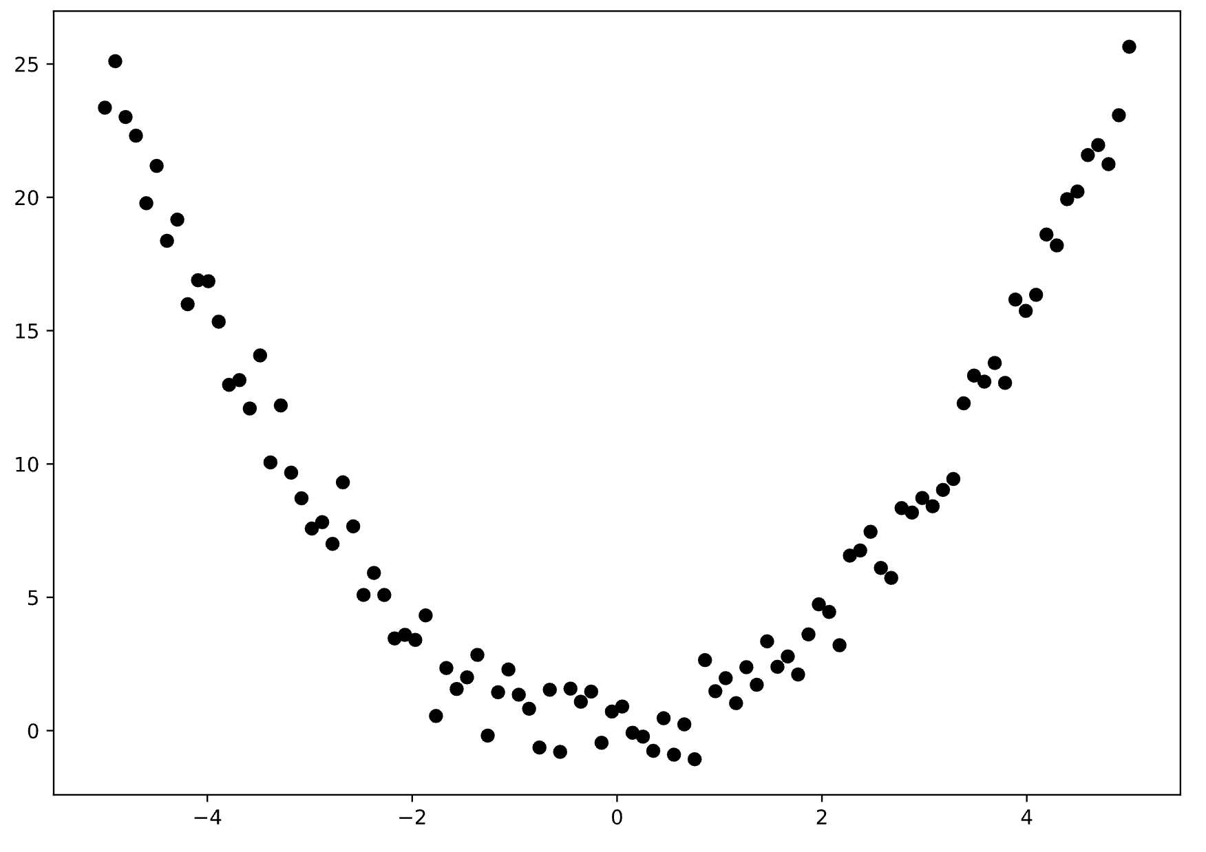
Image 2 - Relationship between X and Y (Image by author)
And that’s your data. Now it’s time to create a model which follows this curve.
Create Your First Artificial Neural Network (ANN) Model in PyTorch
In this section, you’ll create your first neural network for regression in PyTorch. Don’t worry about the code and the technical stuff - the idea is just to get a 10000-foot overview of the subject. The following articles will go over everything in more depth.
A common way to declare a neural network in PyTorch is by writing a custom Python class. It has to inherit from the nn.Module, implement a constructor that calls the constructor from the superclass, and also implement a forward() method that models a forward pass through the network.
You want to declare your network layers in the constructor. The input layer matches the data coming into the network and leaving into the next layer. Our x has only one dimension, so the first argument in nn.Linear() will be 1. The second argument represents the number of output nodes you want. For now, let’s build a stupidly simple network with only 1 output node.
The number of input features in the output must match the number of output features from the previous layer.
The number of output features in the output layer is 1 in this case, since we’re predicting one continuous value.
Further in the forward() method, you’re passing your data through the input layer wrapped by a non-linear activation function. ReLU will do the job pretty well. Then you do the same for the output layer, but without the activation function.
Here’s the entire code:
# Inherits from the nn.Module class
class ANN(nn.Module):
    def __init__(self):
        super().__init__()
        # Input layer - 1 input feature (X is 1-dimensional), 1 output feature
        self.input = nn.Linear(1, 1)
        # Output layer - 1 input feature (n output features from the previous layer)
        #              - 1 output feature (regression, predicting a single value)
        self.output = nn.Linear(1, 1)

    # Forward pass
    def forward(self, x):
        # Non-linear ReLU activation applied to the results of passing through the input layer
        x = F.relu(self.input(x))
        # Output layer - actual prediction - no need to apply an activation function
        x = self.output(x)
        return x
Now it’s time to declare a couple of hyperparameters. The learning_rate represents a scalar by which the gradient will be multiplied when updating the network weights. The n_epochs hyperparameter represents the number of times we’ll go through the entire dataset during model training.
After these, you can instantiate your model class, declare a loss function (measures the error of the model), and the optimizer (implements gradient descent - learning).
Finally, there’s a Python loop that does the training:
# Training parameters
learning_rate = 0.01
n_epochs = 500

# Instantiate the model, loss function (tracks error), and the optimizer (how network learns)
model = ANN()
loss_fun = nn.MSELoss()
optimizer = torch.optim.SGD(model.parameters(), lr=learning_rate)

# Iterate over the number of training epochs
for curr_epoch in range(n_epochs):
    # Forward pass
    pred = model(x)

    # Calculate the loss
    loss = loss_fun(pred, y)

    # Backpropagation
    optimizer.zero_grad()
    loss.backward()
    optimizer.step()
Once the training is finished, you can make a final forward pass through the network to calculate the predictions:
# Make predictions by going through the forward pass once again
predictions = model(x)
This predictions tensor has a gradient function attached to it. Essentially, the tensor is still attached to the computational graph:
# Has the gradient function
predictions[:5]
Here’s what you should see:
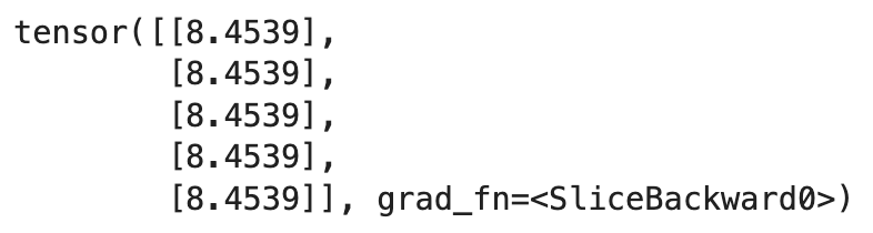
Image 3 - Contents of the predictions tensor (Image by author)
You have to detach it from the graph by calling the detach() function:
# Remove the gradient function
predictions = predictions.detach()
predictions[:5]
Now it’s a plain tensor:
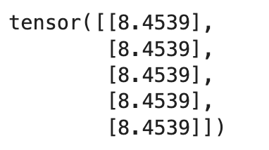
Image 4 - Removing the gradient function (Image by author)
Which means we can visualize it. The additional plt.plot() call will show the predictions as a red line:
# Plot real data against predictions
plt.figure(figsize=(10, 7))

plt.scatter(x, y, c="#000", label="Data")
plt.plot(x, predictions.detach(), c="red", lw=2, label="Predictions")
plt.legend()
plt.show()
Here’s what the actual data and the predicitons look like:
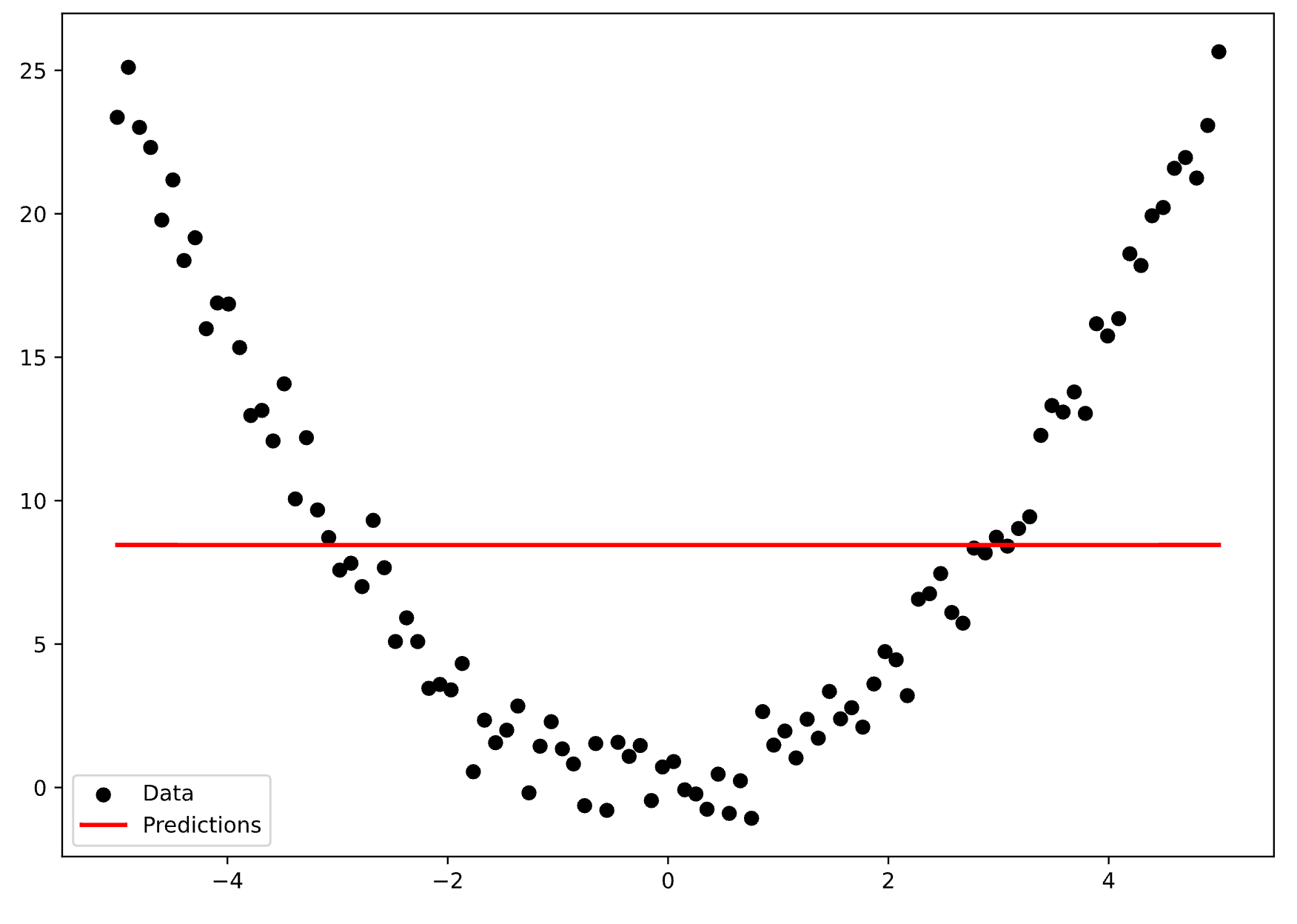
Image 5 - Actual data vs. predictions (1) (Image by author)
That’s something we call underfitting. Your model failed to capture the relationships in the data, which isn’t surprising since the model architecture was way too simple.
Let’s try to find a better fit next.
How to Find The “Right Fit” for a Neural Network in PyTorch
Finding the optimal neural network architecture is more of an art than exact science. It’s quite easy to do on our data, since we can visualize the fit, but you won’t have that luxury on real-world datasets.
So, what can you do? Let’s start by increasing the number of nodes coming out from the input layer, and adding a hidden layer. This will increase the number of parameters and give the network a better chance of getting the predictions right.
Don’t forget to include this new layer in the forward() function:
class ANN(nn.Module):
    def __init__(self):
        super().__init__()
        # Increase the number of output features
        self.input = nn.Linear(1, 16)
        # An additional hidden layer
        self.hidden_1 = nn.Linear(16, 16)
        # Change the number of input features
        self.output = nn.Linear(16, 1)

    def forward(self, x):
        x = F.relu(self.input(x))
        # An additional step in the forward pass
        x = F.relu(self.hidden_1(x))
        x = self.output(x)
        return x
We’ll do the same training and visualizations a couple of more times in the article, so it’s a good idea to write Python functions.
The train_and_evaluate() function will:
- Create a new instance of the
ANN()class - Set up the loss function and the optimizer
- Train the model and calculate predictions
- Calculate the final error after training (Mean squared error)
- Return predictions and MSE
# Regression metric to calculate the model error
from sklearn.metrics import mean_squared_error


# Custom function that instantiates the model and does the training
# Returns the predictions and MSE
def train_and_evaluate(x, y, lr, n_epochs):
    model = ANN()
    loss_fun = nn.MSELoss()
    optimizer = torch.optim.SGD(model.parameters(), lr=lr)

    for curr_epoch in range(n_epochs):
        pred = model(x)
        loss = loss_fun(pred, y)
        optimizer.zero_grad()
        loss.backward()
        optimizer.step()

    predictions = model(x).detach()
    mse = mean_squared_error(y, predictions)

    return predictions.detach(), mse
And the function below - plot_true_vs_predicted() will:
- Plot the actual data as black dots
- Plot predictions as a red line
- Give insights into the final MSE in the chart title
# Custom function to plot the actual vs. predicted data
# Also shows MSE in the title

def plot_true_vs_predictions(x, y, pred, mse):
    plt.figure(figsize=(10, 7))
    plt.scatter(x, y, c="#000", label="Data")
    plt.plot(x, pred, c="red", lw=2, label="Predictions")
    plt.title(f"Acutal vs. predicted; MSE = {mse:.3f}")
    plt.legend()
    plt.show()
Training, evaluation, and visualization now boils to two lines of code:
predictions_ann2, mse_ann2 = train_and_evaluate(x, y, 0.01, 500)
plot_true_vs_predictions(x, y, predictions_ann2, mse_ann2)
Here’s what the network performance looks like now:
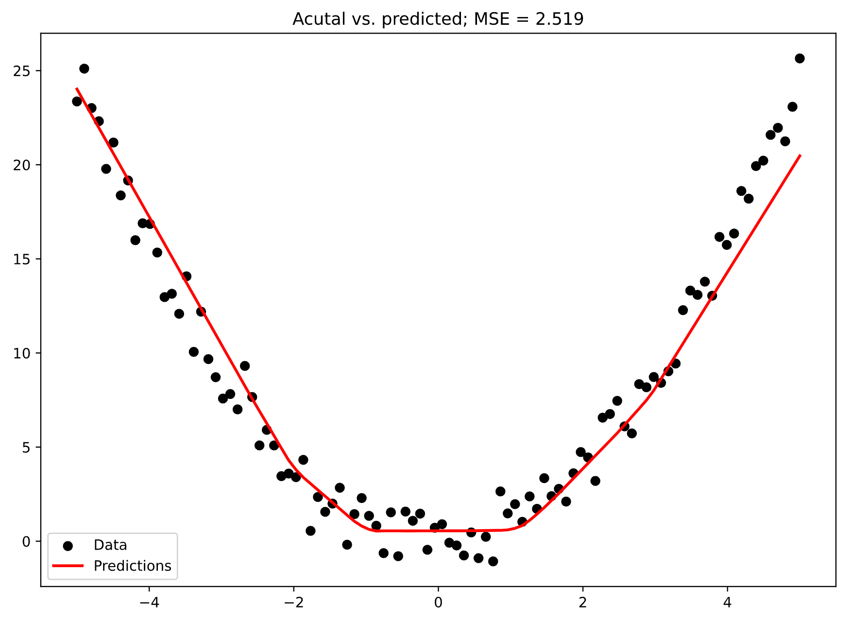
Image 6 - Actual data vs. predictions (2) (Image by author)
This looks like the right fit! The red line overall follows the data correctly and isn’t trying to memorize every point in the dataset. This is the model you should feel confident in using.
But what happens when you keep stacking layers? You get to the opposite end of the spectrum - overfitting.
Common Mistake: Overfitting a Neural Network Model in PyTorch
Overfitting basically means that your model has memorized the training data and fails to generalize on new data. In our case, you should expect to see the line that tries to go through as many data points as possible.
It might seem like a good thing at first, but overfitted models fail to perform well on new data, and have a higher error (i.e. MSE) than models with the right fit.
To demonstrate, let’s stack a couple more hidden layers and increase the number of nodes per layer to something crazy high:
class ANN(nn.Module):
    def __init__(self):
        super().__init__()
        # Just make an overkill with the number of layers and number of nodes per layer
        # This is a simple problem and this network is way too complex
        self.input = nn.Linear(1, 64)
        self.hidden_1 = nn.Linear(64, 64)
        self.hidden_2 = nn.Linear(64, 512)
        self.hidden_3 = nn.Linear(512, 512)
        self.hidden_4 = nn.Linear(512, 64)
        self.output = nn.Linear(64, 1)

    def forward(self, x):
        # Don't forget to include them into the forward pass
        x = F.relu(self.input(x))
        x = F.relu(self.hidden_1(x))
        x = F.relu(self.hidden_2(x))
        x = F.relu(self.hidden_3(x))
        x = F.relu(self.hidden_4(x))
        x = self.output(x)
        return x
We’re dealing with a simple parabola-like dataset, so injecting this many layers and nodes will result in a too-complex of a model.
Let’s train it and visualize the results:
predictions_ann3, mse_ann3 = train_and_evaluate(x, y, 0.01, 1000)
plot_true_vs_predictions(x, y, predictions_ann3, mse_ann3)
Overall, you can see how the line isn’t smooth anymore:
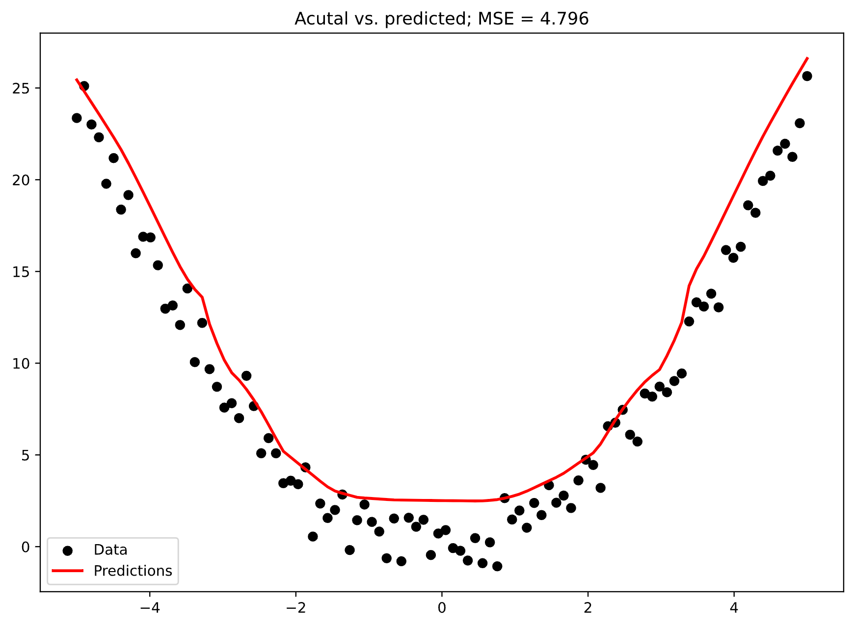
Image 7 - Actual data vs. predictions (3) (Image by author)
Further, MSE increased from 2.5 to 4.8, which is almost double! Even if you couldn’t visualize the fit, the basic mathematics can tell you which model performs better.
Summing up Introduction to Regression in PyTorch
Long story short - simple problems require simple solutions. You can kill a mosquito with a sledgehammer, but you’ll do more harm than good. The same holds true in deep learning.
The following one will show you how to train classification models with PyTorch. Now, we haven’t talked about train/validation/test split, cross-validation and other must-implement techniques when training deep learning models. We’ll cover these topics two articles from now.
I wanted to provide a 10000-foot overview first and show you how to train models with PyTorch before diving into the nitty-gritty details.
Stay tuned to Better Data Science for more.