Simple Classification with Artificial Neural Networks (ANN) in PyTorch
Supervised machine learning encompasses regression and classification tasks. I’ve already covered how to do regression with PyTorch, so this article will focus on classification. To be more specific, you’ll learn how to train and evaluate a binary classifier on a synthetic dataset.
This article will also teach you how to visualize the decision boundary of a classification neural network - something that will come in handy when data dimensionality allows it.
Once again - this is not a comprehensive guide on the subject. You won’t learn what’s behind every PyTorch function. I’ll have dedicated articles for each, but for now, it’s enough to grasp a high-level overview.
Table of contents:
How to Create a Synthetic Classification Dataset in PyTorch
There are many real classification datasets online, so why are we creating a synthetic one? The reason is simple - it won’t skew the focus point of the article on data preprocessing, and it will allow us to visualize the patterns the neural network has learned.
But first - the library import. You have all of these packages on your system if you’ve gone through the PyTorch installation article:
import numpy as np

import torch
import torch.nn as nn
import torch.nn.functional as F

import matplotlib.pyplot as plt
import matplotlib_inline
matplotlib_inline.backend_inline.set_matplotlib_formats("svg")
Onto the dataset. I’ll create it by using the make_circles() function from Scikit-Learn. This function makes N circles in two distinct classes. The noise argument adds some noise to the data points, so you don’t get a perfect circle back.
The following code snippet creates a 2-dimensional tensor of 500 data points (X), and a 1-dimensional tensor of class labels (y):
from sklearn.datasets import make_circles

# Number of data points
n = 500

# Just a small amount of noise for easier classification
X, y = make_circles(n_samples=n, noise=0.02)

# Convert to tensors
X = torch.tensor(X, dtype=torch.float)
y = torch.tensor(y, dtype=torch.float).reshape(n, -1)
Let’s print the first couple of entries from both to see what they look like:
X[:5], y[:5]
You’ll get different values, but here are mine:
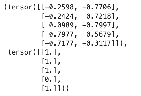
Image 1 - Contents of the X and y tensors (Image by author)
The goal of the classification neural network model will be to predict either 0 or 1 (y) based on the two input features (X).
It shouldn’t be too difficult of a task, since the data points are clearly separable:
plt.figure(figsize=(10, 7))

plt.scatter(X[:, 0][np.where(y == 0)[0]], X[:, 1][np.where(y == 0)[0]], c="blue", label="Class 1")
plt.scatter(X[:, 0][np.where(y == 1)[0]], X[:, 1][np.where(y == 1)[0]], c="red", label="Class 2")
plt.legend()
plt.show()
Here’s what they look like visually:
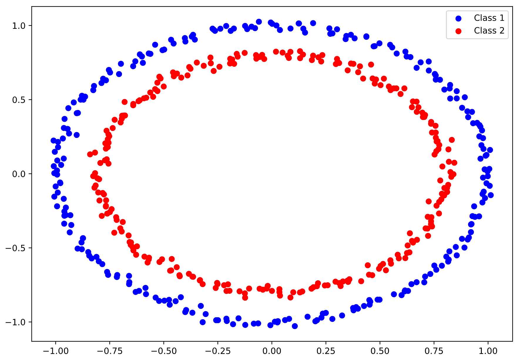
Image 2 - Circular dataset with two classes (Image by author)
The separation is visible, but can a neural network detect it? How complex of an architecture do you need? Let’s find out next.
Write a Simple ANN for Binary Classification
The goal of this section is to write the most basic neural network classification model with PyTorch, declare a couple of helper functions for model training and visualization, and see how our network performs.
Just like in the regression article, the idea is to use a Python class for the network. We’ll have an input layer with 2 input features (since X has two dimensions) and 2 output features (random).
The output layer of the network will have only 1 output node. We don’t need more since we’re doing binary classification, and the model will return a prediction probability.
It’s mandatory that you don’t wrap the output layer with any activation function! The loss function will implement the Sigmoid activation function, so you don’t have to move a muscle.
Here’s the entire code snippet for the model class:
class ANN(nn.Module):
    def __init__(self):
        super().__init__()
        self.input = nn.Linear(2, 2)
        # It's a good practice to have 1 output node - binary classification
        self.output = nn.Linear(2, 1)

    def forward(self, x):
        x = F.relu(self.input(x))
        x = self.output(x)
        return x
Up next, I’ll write a couple of helper functions that we’ll reuse through the article.
Helper Functions
The first helper function is responsible for training and evaluating a model on a set of data (X) and labels (y).
It instantiates the model class, tracks loss through BCEWithLogitsLoss(), uses stochastic gradient descent (SGD) during backpropagation to update the weights, trains the model, and returns the prediction classes and the accuracy score.
The code snippet has comments in critical places, so you shouldn’t have trouble understanding it:
# Measure the performance with accuracy
from sklearn.metrics import accuracy_score


def train_and_evaluate(X, y, lr, n_epochs):
    model = ANN()
    # BCEWithLogitsLoss() implements the Sigmoid function for us
    loss_fun = nn.BCEWithLogitsLoss()
    optimizer = torch.optim.SGD(model.parameters(), lr=lr)

    for curr_epoch in range(n_epochs):
        pred = model(X)
        loss = loss_fun(pred, y)
        optimizer.zero_grad()
        loss.backward()
        optimizer.step()

    # Get the prediction probabilities
    prediction_probas = model(X).detach()
    # BCEWithLogitsLoss turns class 0 to below 0 and class 1 to above 0
    predictions = (prediction_probas > 0).float()
    acc = accuracy_score(y, predictions)

    return model, predictions.detach(), acc
The next function plots the decision boundary of a binary classifier. This will be useful to visually inspect the thinking of a neural network model, and visually confirm if the model gets it.
I’ve borrowed and modified the code from Prudvi RajKumar’s article on Medium to work with our dataset:
def plot_decision_boundary_contour(model, X, y, acc):
    # Inspiration - https://medium.com/@prudhvirajnitjsr/simple-classifier-using-pytorch-37fba175c25c

    x_min, x_max = X[:, 0].min().item() - .5, X[:, 0].max().item() + .5
    y_min, y_max = X[:, 1].min().item() - .5, X[:, 1].max().item() + .5
    h = 0.01

    # Coordinate matrices
    xx, yy = np.meshgrid(np.arange(x_min, x_max, h), np.arange(y_min, y_max, h))
    tensor_for_pred = torch.tensor(np.c_[xx.ravel(), yy.ravel()], dtype=torch.float32)
    Z = model(tensor_for_pred).detach().reshape(xx.shape)
    Z_classes = (Z > 0).float()

    plt.figure(figsize=(10, 7))
    plt.title(f"Accuracy = {100 * acc}%")
    plt.contourf(xx, yy, Z_classes, cmap=plt.cm.Spectral)
    plt.scatter(X[:, 0], X[:, 1], c=y, cmap=plt.cm.binary)
Let’s now apply these two functions on the ANN class.
Evaluating Your First Model
The only thing left to do is to train the model and show its predictive performance. The following two lines of code leverage the previously written helper functions:
model, predictions, acc = train_and_evaluate(X, y, 0.01, 500)
plot_decision_boundary_contour(model, X, y, acc)
This is the output I got:
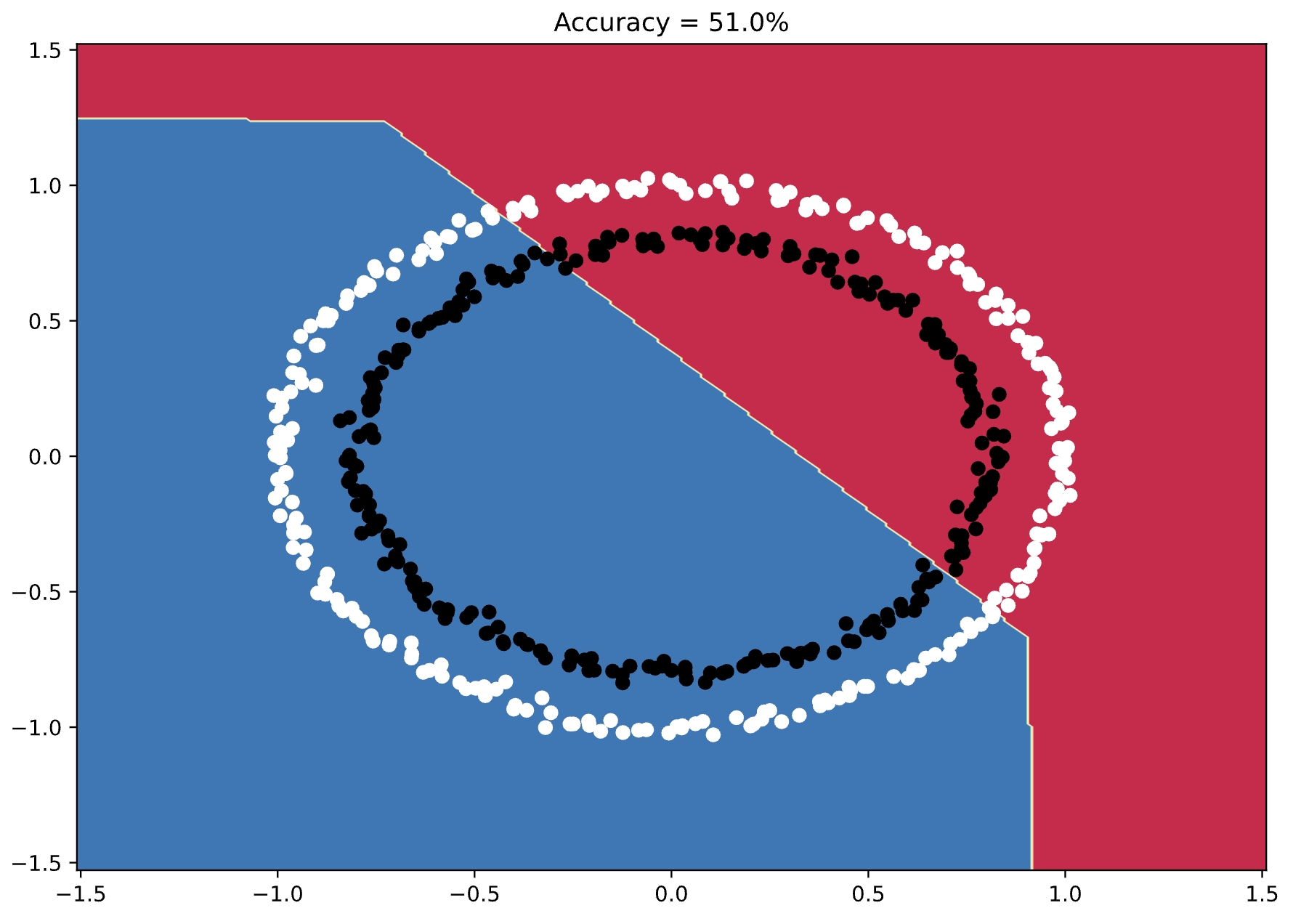
Image 3 - Model’s decision boundary (1) (Image by author)
Long story short - the neural network model doesn’t get it. The decision boundary looks random, and the accuracy is only 51%.
A model that only generates a random number would have an accuracy of 50%, so we have some work to do.
How to Find the Right Network Architecture for Binary Classification
The idea of this section is to see what happens to the model accuracy and decision boundary as we increase the number of layers and the number of units per layer.
There’s definitely a sweet spot for our dataset, and finding it boils down to experimentation.
Just-Right Fit
We should be able to get a highly-accurate model since the data is clearly separable and doesn’t contain much noise.
The following model architecture continuously gave me high accuracy, all while keeping the training time short:
class ANN(nn.Module):
    def __init__(self):
        super().__init__()
        # Increase the number of units significantly
        self.input = nn.Linear(2, 1024)
        # Add a hidden layer
        self.hidden_1 = nn.Linear(1024, 1024)
        self.output = nn.Linear(1024, 1)

    def forward(self, x):
        x = F.relu(self.input(x))
        x = F.relu(self.hidden_1(x))
        x = self.output(x)
        return x
As you can see, it adds one hidden layer and drastically increases the number of nodes in the layers.
Let’s train it and plot the decision boundary:
model2, predictions2, acc2 = train_and_evaluate(X, y, 0.01, 500)
plot_decision_boundary_contour(model2, X, y, acc2)
Here’s what it looks like:
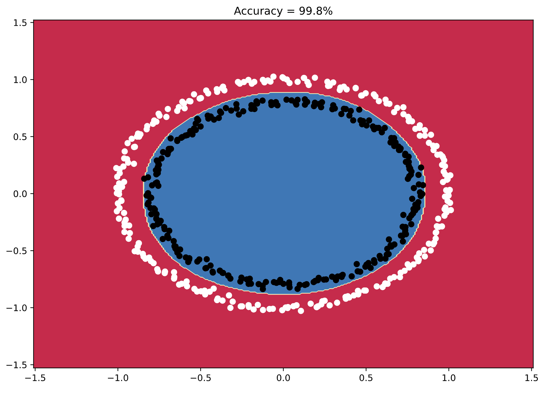
Image 4 - Model’s decision boundary (2) (Image by author)
Almost 100% accuracy! You can see how the neural network thinks when classifying these numbers, and how the decision boundary almost perfectly follows the shape of the data points.
That’s the sweet spot for this dataset, but let’s try adding more layers to see what happens.
Overfitted Model
Overfitting means that your model has memorized the training data and fails to generalize on new data.
Increasing the model complexity too much is a guaranteed way to introduce overfitting, which will reduce the accuracy as a result.
The following network architecture adds one more hidden layer, and somewhat changes the number of nodes per layer:
class ANN(nn.Module):
    def __init__(self):
        super().__init__()
        # More layers and nodes per layer
        self.input = nn.Linear(2, 512)
        self.hidden_1 = nn.Linear (512, 1024)
        self.hidden_2 = nn.Linear(1024, 512)
        self.output = nn.Linear(512, 1)

    def forward(self, x):
        x = F.relu(self.input(x))
        x = F.relu(self.hidden_1(x))
        x = F.relu(self.hidden_2(x))
        x = self.output(x)
        return x
Let’s train it to see the results:
model3, predictions3, acc3 = train_and_evaluate(X, y, 0.01, 500)
plot_decision_boundary_contour(model3, X, y, acc3)
Here’s what I got:
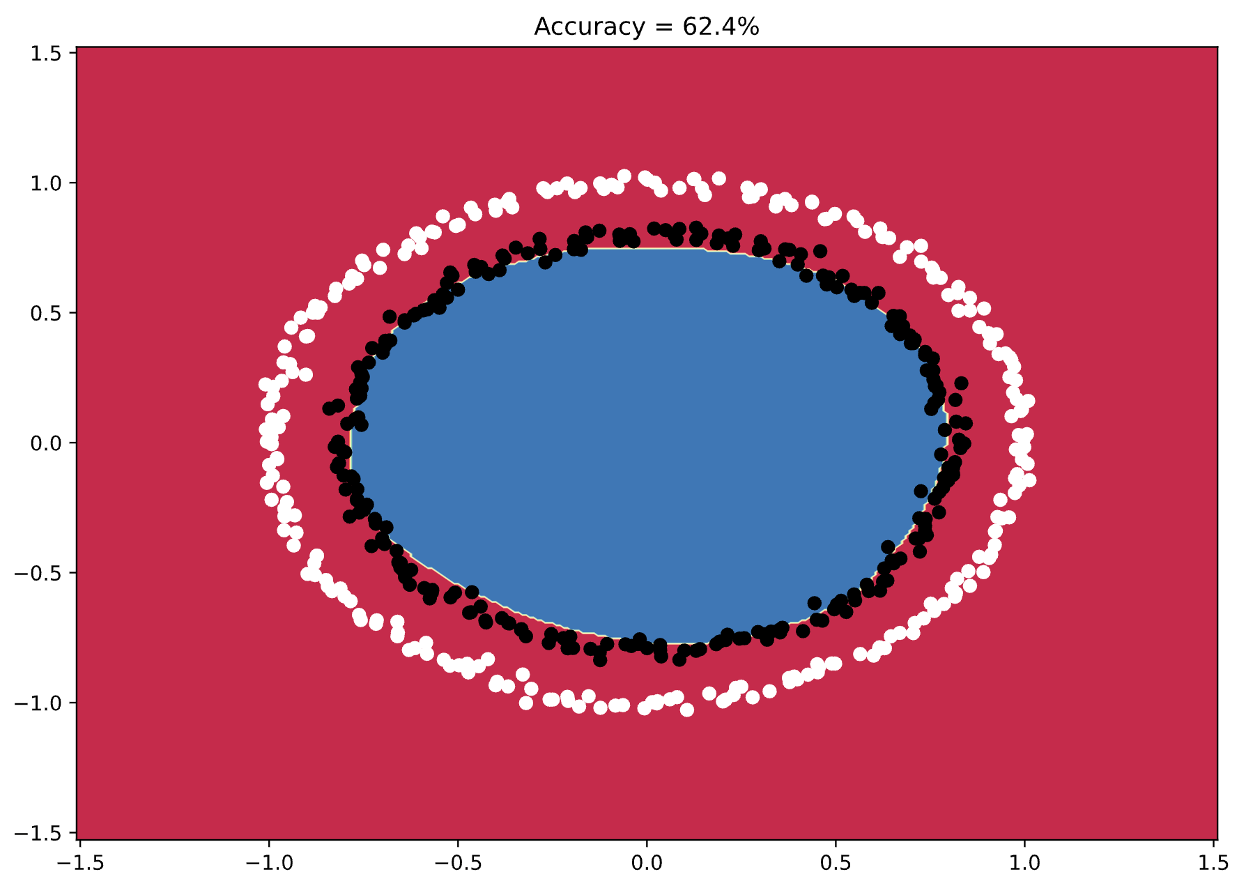
Image 5 - Model’s decision boundary (3) (Image by author)
You can see from the decision boundary how the model just barely fails to make the correct classifications. It looks similar to the previous chart, but many instances are just outside the boundary.
That’s overfitting for you.
Summing up PyTorch Classification with ANNs
Building a binary classifier in PyTorch boils down to creating a model class and picking the right set of hyperparameters. You’ve seen how the architecture impacts predictive performance - remember to test a couple of options to see what works for you.
Typically, don’t go to extremes with the number of model parameters. Too low a number leads to underfitting while too high a number leads to overfitting. There’s usually a sweet spot in between.
The following article will dive deep into train/validation/test split in deep learning and PyTorch, which is a must-know concept for testing if your model generalizes or not.
Stay tuned to Better Data Science for more.