
You’ll need 10 minutes to implement pooling with strides in Python and Numpy
The previous TensorFlow article showed you how to write convolutions from scratch in Numpy. Now it’s time to discuss pooling, a downscaling operation that usually follows a convolutional layer. You want to know a secret? It’s not rocket science to implement from scratch.
After reading, you’ll know what pooling and strides are and how to write them from scratch in Numpy. You’ll get an intuitive understanding first, and then apply it in Python. When that’s out of the way, you’ll apply pooling to a real image and compare results with TensorFlow’s pooling layer to see if we did anything wrong. Spoiler alert: we didn’t.
The code you’ll see today isn’t optimized for speed, but instead for maximum readability and ease of understanding.
Don’t feel like reading? Watch my video instead:
How Pooling Works
The pooling operation usually follows the convolution layer. Its task is to reduce the dimensionality of the result coming in from the convolutional layer by keeping what’s relevant and discarding the rest.
The process is simple — you define an n x n region and stride size. The region represents a small matrix that slides over the image and works with individual pools. A pool is just a fancy word for a small matrix on the convolutional output from which, most commonly, the maximum value is kept. A good starting value for the region size is 2x2.
The stride represents the number of pixels to the right the region moves after completing a single step. When the region reaches the end of the first row blocks, it moves down by a stride size and repeats the process. A good starting value for the stride is 2. Opting for a stride size lower than 2 doesn’t make much sense, as you’ll see shortly.
The most common type of pooling is Max Pooling, which means only the highest value of a region is kept. You’ll sometimes encounter Average Pooling, but not nearly as often. Max pooling is a good place to start because it keeps the most activated pixels (ones with the highest values) and discards the rest. On the other hand, averaging would even out the values. You don’t want that most of the time.
While we’re on the topic of how pooling works, let’s see what happens to a small 4x4 matrix when you apply max pooling to it. We’ll use a region size of 2x2 and the stride size of 1:
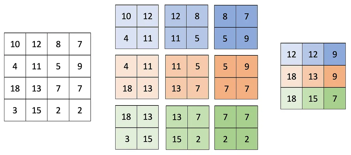
Image 1 — Max Pooling with the region size of 2x2 and the stride size of 1 (image by author)
A total of 9 pools was extracted from the input matrix, and only the largest value from each pool was kept. As a result, pooling reduced the dimensionality by a single pixel in height and width. That’s why opting for a stride size lower than 2 makes no sense, as pooling just barely reduced the dimensionality.
Let’s apply the pooling operation once again, but this time with a stride size of 2 pixels:
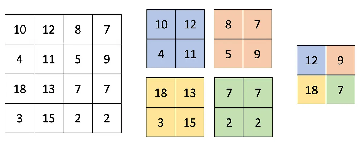
Image 2 — Max Pooling with the region size of 2x2 and the stride size of 2 (image by author)
Much better — we now had only four pools to work with, and we got rid of half the pixels in height and width.
Next, let’s see how to implement the pooling logic from scratch in Python.
MaxPooling From Scratch in Python and Numpy
Now the fun part begins. Let’s start by importing Numpy and declaring the matrix from the previous section:
import numpy as np

conv_output = np.array([
    [10, 12,  8,  7],
    [ 4, 11,  5,  9],
    [18, 13,  7,  7],
    [ 3, 15,  2,  2]
])
conv_output
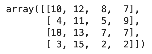
Image 3 — Dummy convolutional output matrix (image by author)
To make things easier to follow, I’ll split this section into two parts. The first one shows you how to extract pools from a matrix.
Extract Pools From a Matrix
To start, you’ll have to select values for two parameters —pool size, and stride size. You already know what these represent, and we’ll stick with the common values of 2x2 and 2, respectively. To extract individual pools, you’ll have to:
- Iterate over all rows with a step size of 2.
- Iterate over all columns with a step size of 2.
- Get a single pool by slicing the input matrix.
- Ensure it has a correct shape — 2x2 in our case.
In code, it boils down to the following:
# Define paramters
pool_size = 2
stride = 2

# For all rows with the step size of 2 (row 0 and row 2)
for i in np.arange(conv_output.shape[0], step=stride):
    # For all columns with the step size of 2 (column 0 and column 2)
    for j in np.arange(conv_output.shape[0], step=stride):
        # Get a single pool
        # First  - Image[0:2, 0:2] -> [[10, 12], [ 4, 11]]
        # Second - Image[0:2, 2:4] -> [[ 8,  7], [ 5,  9]]
        # Third  - Image[2:4, 0:2] -> [[18, 13], [ 3, 15]]
        # Fourth - Image[2:4, 2:4] -> [[ 7,  7], [ 2,  2]]
        mat = conv_output[i:i+pool_size, j:j+pool_size]

        # Ensure that the shape of the matrix is 2x2 (pool size)
        if mat.shape == (pool_size, pool_size):
            # Print it
            print(mat)
    # Print a new line when the code reaches the end of a single row block
    print()

Image 4 — Extracted pools with a pool size of 2x2 and stride size of 2 (image by author)
Easy, right? There are four pools in total, just as we had in the previous section. Let’s see what happens if we reduce the stride size to 1 and keep everything else as is:
pool_size = 2
stride = 1

for i in np.arange(conv_output.shape[0], step=stride):
    for j in np.arange(conv_output.shape[0], step=stride):
        mat = conv_output[i:i+pool_size, j:j+pool_size]
        if mat.shape == (pool_size, pool_size):
            print(mat)
    print()
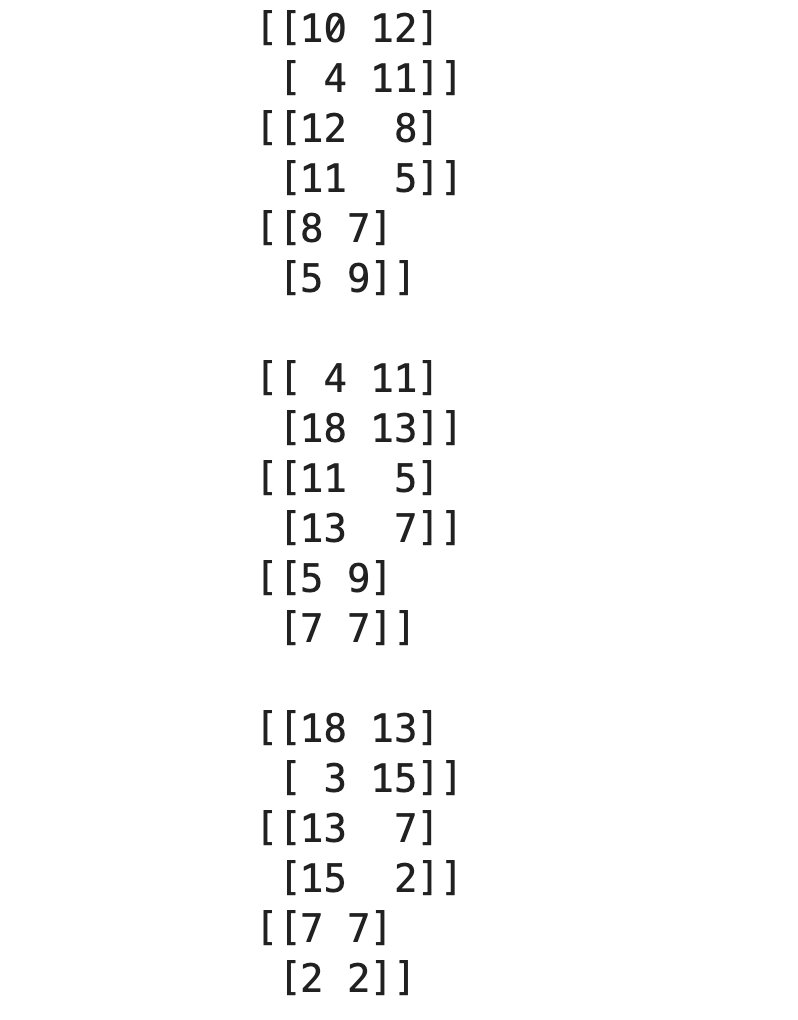
Image 5 — Extracted pools with a pool size of 2x2 and stride size of 1 (image by author)
We have nine pools here, as expected. Our pooling logic works! Let’s wrap it into a single function next:
def get_pools(img: np.array, pool_size: int, stride: int) -> np.array:
    # To store individual pools
    pools = []

    # Iterate over all row blocks (single block has `stride` rows)
    for i in np.arange(img.shape[0], step=stride):
        # Iterate over all column blocks (single block has `stride` columns)
        for j in np.arange(img.shape[0], step=stride):

            # Extract the current pool
            mat = img[i:i+pool_size, j:j+pool_size]

            # Make sure it's rectangular - has the shape identical to the pool size
            if mat.shape == (pool_size, pool_size):
                # Append to the list of pools
                pools.append(mat)

    # Return all pools as a Numpy array
    return np.array(pools)
And do a final test to double-check:
test_pools = get_pools(img=conv_output, pool_size=2, stride=2)
test_pools
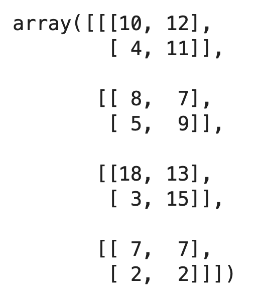
Image 6 — Testing the get_pools() function (image by author)
It’s confirmed — our function works as expected. The question remains — how can we implement the max pooling algorithm now?
Implement Max Pooling From Scratch
So what, we now have to take the maximum value from each pool? Well, it’s a bit more complex than that. Here’s a list of tasks you’ll need to implement:
- Get the total number of pools — it’s simply the length of our pools array.
- Calculate the target shape — image size after performing the pooling operation. It’s calculated as the square root of the number of pools cast as an integer. For example, if the number of pools is 16, we need a 4x4 matrix — the square root of 16 is 4.
- Iterate over all pools, get the maximum value and append it to the list.
- Return the list as a Numpy array reshaped to the target size.
Sounds like a lot, but it boils down to seven lines of code (comments excluded):
def max_pooling(pools: np.array) -> np.array:
    # Total number of pools
    num_pools = pools.shape[0]
    # Shape of the matrix after pooling - Square root of the number of pools
    # Cast it to int, as Numpy will return it as float
    # For example -> np.sqrt(16) = 4.0 -> int(4.0) = 4
    tgt_shape = (int(np.sqrt(num_pools)), int(np.sqrt(num_pools)))
    # To store the max values
    pooled = []

    # Iterate over all pools
    for pool in pools:
        # Append the max value only
        pooled.append(np.max(pool))

    # Reshape to target shape
    return np.array(pooled).reshape(tgt_shape)
That’s it — let’s test it on our array of four pools:
max_pooling(pools=test_pools)
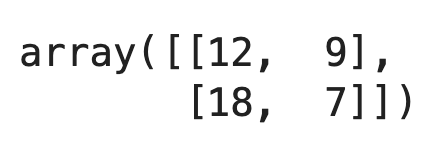
Image 7 — Max pooling results (image by author)
Works like a charm! Let’s test our functions on a real image next to see if anything breaks.
Max Pooling From Scratch on a Real Image
To start, import PIL and Matplotlib for easy image visualization. We’ll also declare two functions for showing images — the first one displays a single image, and the second one displays two images side by side:
from PIL import Image, ImageOps
import matplotlib.pyplot as plt

def plot_image(img: np.array):
    plt.figure(figsize=(6, 6))
    plt.imshow(img, cmap='gray');

def plot_two_images(img1: np.array, img2: np.array):
    _, ax = plt.subplots(1, 2, figsize=(12, 6))
    ax[0].imshow(img1, cmap='gray')
    ax[1].imshow(img2, cmap='gray');
We’ll use the Dogs vs. Cats dataset from Kaggle for the rest of the article. It’s licensed under the Creative Commons License, which means you can use it for free. One of the previous articles described how to preprocess it, so make sure to copy the code if you want to follow along on identical images.
That’s not a requirement, since you can apply pooling to any image. Seriously, download any image from the web, it will serve you just fine for today. In reality, pooling almost always follows a convolutional layer, but we’ll apply it directly to an image to keep things extra simple.
The code snippet below loads in a sample cat image from the training set, grayscales it, and resizes it to 224x224 pixels. The transformations aren’t mandatory, but will make our job easier, as there’s only one color channel to apply pooling to:
img = Image.open('data/train/cat/1.jpg')
img = ImageOps.grayscale(img)
img = img.resize(size=(224, 224))
plot_image(img=img)
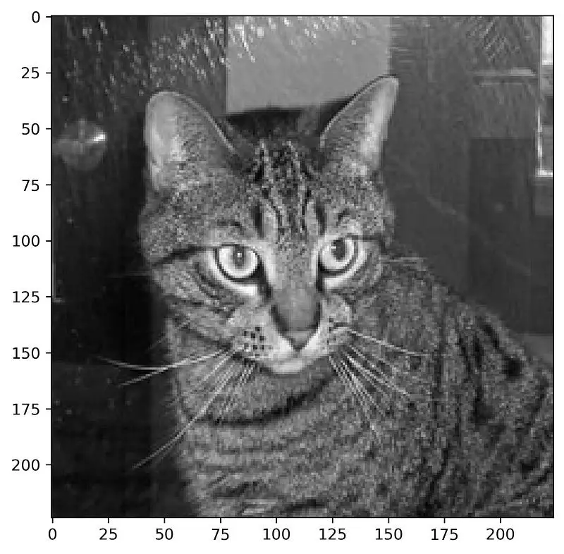
Image 8 — Random cat image from the training set (image by author)
We can now extract individual pools. Remember to convert the image to a Numpy array first. We’ll keep the pool size and stride size parameters at 2:
cat_img_pools = get_pools(img=np.array(img), pool_size=2, stride=2)
cat_img_pools
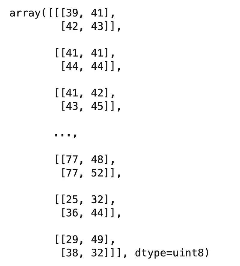
Image 9 — Individual pools extracted from the cat image (image by author)
Let’s see how many pools there are in total:

Image 10 — Number of individual pools and their shape
We have 12,544 pools in total, each being a small 2x2 matrix. The shape makes sense, as the square root of 12,544 is 112. Put simply, our cat image will be of size 112x112 pixels after the pooling operation.
There’s nothing left to do except apply the max pooling:
cat_max_pooled = max_pooling(pools=cat_img_pools)
cat_max_pooled
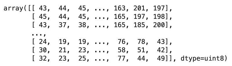
Image 11 — Cat image in a matrix format after max pooling (image by author)
We’ll display the pooled image in a bit, but let’s verify the shape is indeed 112x112 pixels first:

Image 12 — Shape of the pooled cat image (image by author)
Everything looks right, so let’s display the cat images before and after pooling side by side:
plot_two_images(img1=img, img2=cat_max_pooled)
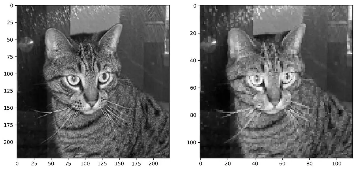
Image 13 — Cat image before and after max pooling (image by author)
Keep in mind that the image on the right is displayed in the same size as the image on the left, even though it’s smaller. Check the X and Y axis labels for both images to verify.
To summarize — the max pooling operation drastically reduced the number of pixels, but we can still easily classify it as a cat. Reducing the number of pixels in convolutional layers will reduce the number of parameters in the network, and hence reduce the model complexity and training time.
There’s still one question left to answer —how do we know we did everything correctly? That’s what the following section answers.
Verification — Max Pooling With TensorFlow
You can apply TensorFlow’s max pooling layer directly to an image without training the model first. That’s the best way to examine if we did everything correctly in the previous sections. To start, import TensorFlow and declare a sequential model with a single max pooling layer only:
import tensorflow as tf

model = tf.keras.Sequential([
    tf.keras.layers.MaxPool2D(pool_size=2, strides=2)
])
You’ll have to reshape the cat image before passing it through the model. TensorFlow expects a 4-dimensional input, so you’ll have to add two additional dimensions alongside the image height and width:
cat_arr = np.array(img).reshape(1, 224, 224, 1)
cat_arr.shape
Image 14 — TensorFlow approved image shape (image by author)
And now comes the fun part — you can use TensorFlow’s predict() function without training the model first. Just pass in a single image and reshape the result back to a 112x112 matrix:
output = model.predict(cat_arr).reshape(112, 112)
output
Image 15 — Cat image after applying Max pooling with TensorFlow (image by author)
The matrix looks familiar, but let’s not jump to conclusions. You can use the array_equal() function from Numpy to test if all elements from two arrays are identical. The code snippet below uses it to compare our from-scratch pooling result with TensorFlow’s output:
np.array_equal(cat_max_pooled, output)
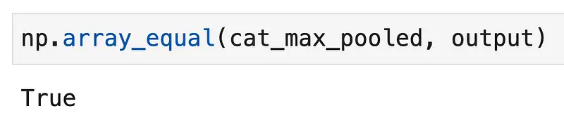
Image 16 — Checking for array equality (image by author)
Who would tell — Pooling isn’t a black box after all. The outputs are identical, which means our from-scratch implementation is fully functional. Does that mean you should use it for your daily computer vision tasks? Absolutely not, and there’s a good reason why.
Conclusion
You now know how to implement convolutions and pooling from scratch in Python and Numpy. It’s a big achievement, but it doesn’t mean you should write your deep learning framework from scratch. TensorFlow is highly optimized, and our from-scratch implementation isn’t. My goal was to write an understandable code, and that comes with a lot of loops and time-consuming operations. In a nutshell, our approach sacrificed efficiency for readability.
Don’t bother with from-scratch implementations in real-world projects. These are here to get a better understanding of relatively easy concepts.
Stay tuned for the next article in which we’ll implement a more robust and accurate image classifier with TensorFlow.
Stay connected
- Sign up for my newsletter
- Subscribe on YouTube
- Connect on LinkedIn