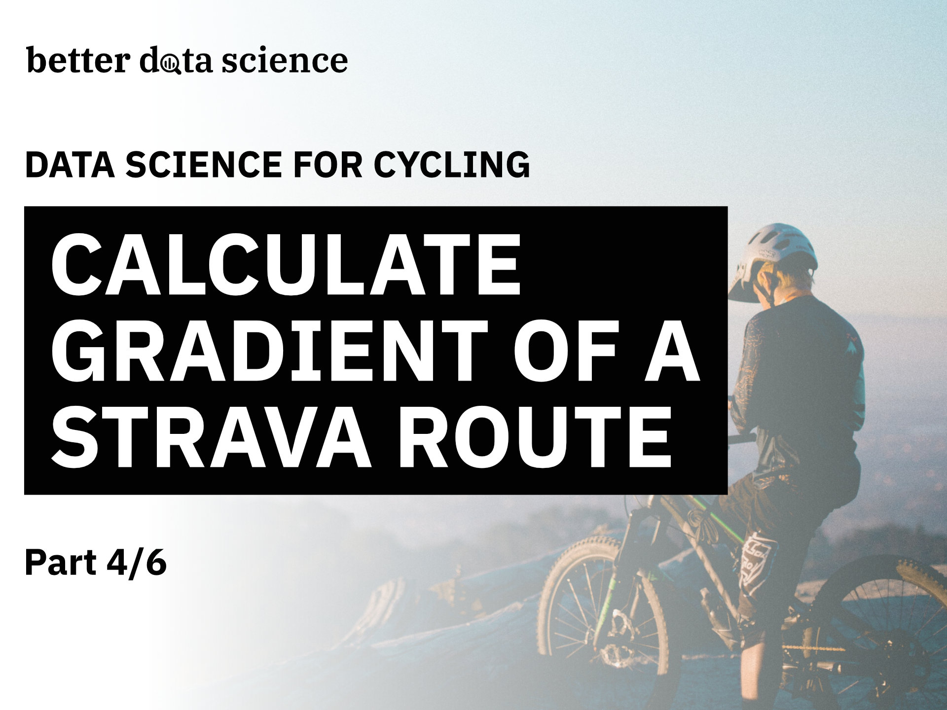
Part 4/6 - Calculate and visualize gradients of a Strava route GPX files with Python
Last week you’ve seen how easy it is to calculate the elevation difference and distance of a Strava route. It was a step in the right direction, as you’ll need both elevation and distance data today. One thing cyclists love talking about is gradients. These represent the slope of the surface you’re riding on.
As it turns out, you can estimate them effortlessly with basic Python and math skills. We have a lot to cover today, so let’s dive straight in.
Don’t feel like reading? Watch my video instead:
You can download the source code on GitHub.
How to Read a Strava Route Dataset
We won’t bother with GPX files today, as we already have route data points, elevation, and distance extracted to a CSV file. To start, import the usual suspects and tweak Matplotlib’s default styling:
import numpy as np
import pandas as pd
import matplotlib.pyplot as plt

plt.rcParams['figure.figsize'] = (16, 6)
plt.rcParams['axes.spines.top'] = False
plt.rcParams['axes.spines.right'] = False
From here, load the route dataset:
route_df = pd.read_csv('../data/route_df_elevation_distance.csv')
route_df.head()
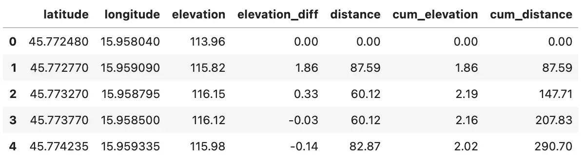
Image 1 - Strava route dataset with distance and elevation data (image by author)
Read the last week’s article if you don’t have the route dataset in this format. To recap, there are 835 data points in total on this 36,4-kilometer route, so there are on average 43,6 meters between data points.
We can use the elevation difference and distance data to estimate average gradients on each of 835 individual segments.
How to Calculate Gradient from a Strava Route
A gradient is nothing but a slope of the surface you’re riding on. Our data is quite limited, as we only have 835 data points spread over 36 kilometers. We’ll do our best, but everything you’ll see from this point is just an estimation.
We can estimate the average gradient between two data points by dividing the elevation difference between them with the distance covered and multiplying the results by 100.
Let’s test the logic with hardcoded values from the second data point (1.86 meters of elevation gained over 87.59 meters):
(1.86 / 87.59) * 100

>>> 2.1235300833428474
The average grade from the route start to the second data point was 2.1%. This means that, provided the same gradient continues, you would gain 2.1 meters of elevation after 100 meters of distance.
It’s only an average, so keep that in mind. The first 15 meters of the segment could have a 10% gradient, and the remaining 72 meters could be completely flat. On the other hand, the entire 87-meter segment could have a perfectly distributed 2.1% grade. The point is - we can’t know for sure, and the above logic is the best we can do.
Let’s apply it to the entire dataset. We’ll skip the first row, as there’s nothing to compare it with. Gradients are usually rounded up to single decimal points, but that’s a convention, not a requirement. Feel free to include more.
gradients = [np.nan]

for ind, row in route_df.iterrows():
    if ind == 0:
        continue
    grade = (row['elevation_diff'] / row['distance']) * 100
    gradients.append(np.round(grade, 1))

gradients[:10]

Image 2 - First ten estimated gradients (image by author)
Calculations done - let’s now visualize the average gradient for each of the 835 data points:
plt.title('Terrain gradient on the route', size=20)
plt.xlabel('Data point', size=14)
plt.ylabel('Gradient (%)', size=14)
plt.plot(np.arange(len(gradients)), gradients, lw=2, color='#101010');
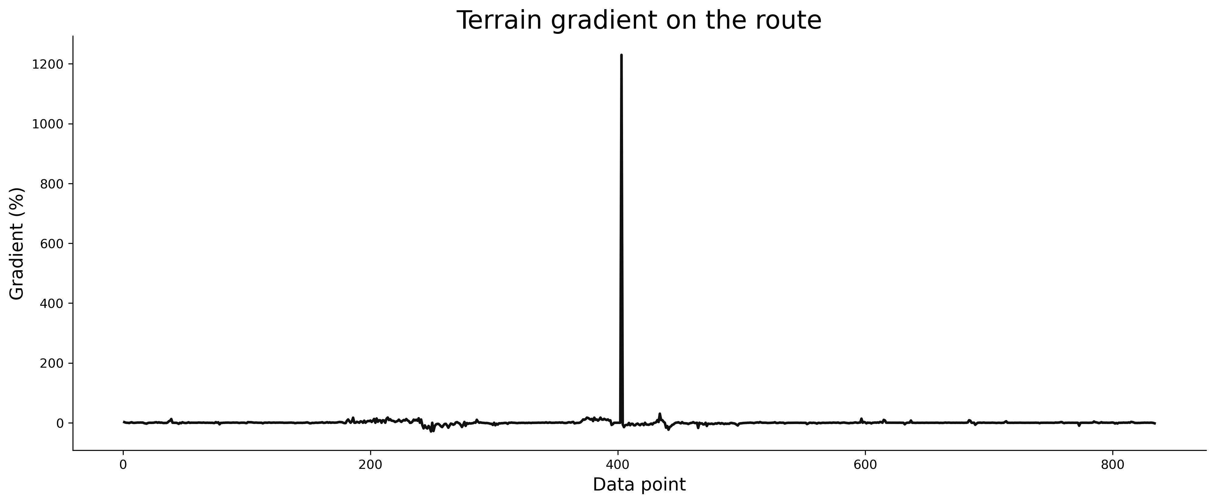
Image 3 - Estimated average route gradient v1 (image by author)
There appears to be something wrong with the route file. A single data point has over 1200% gradient, which is impossible. In theory, that would mean you gain 1200 meters of elevation after 100 meters of distance.
We’ll mitigate this issue by adding a condition - if the estimated average gradient is greater than 30%, we’ll append NaN to the list. There are no gradients above 30% on this route, and such gradients are extremely rare overall.
gradients = [np.nan]

for ind, row in route_df.iterrows():
    if ind == 0:
        continue

    grade = (row['elevation_diff'] / row['distance']) * 100

    if grade > 30:
        gradients.append(np.nan)
    else:
        gradients.append(np.round(grade, 1))
Let’s see how it looks like:
plt.title('Terrain gradient on the route', size=20)
plt.xlabel('Data point', size=14)
plt.ylabel('Gradient (%)', size=14)
plt.plot(np.arange(len(gradients)), gradients, lw=2, color='#101010');

Image 4 - Estimated average route gradient v2 (image by author)
It’s a step in the right direction, but we now have a couple of missing data points. The thing is - there’s a stupidly simple fix.
How to Interpolate Incorrect Gradients From a Strava Route
First things first, we’ll assign the calculated gradients to a new dataset column:
route_df['gradient'] = gradients
route_df.head()
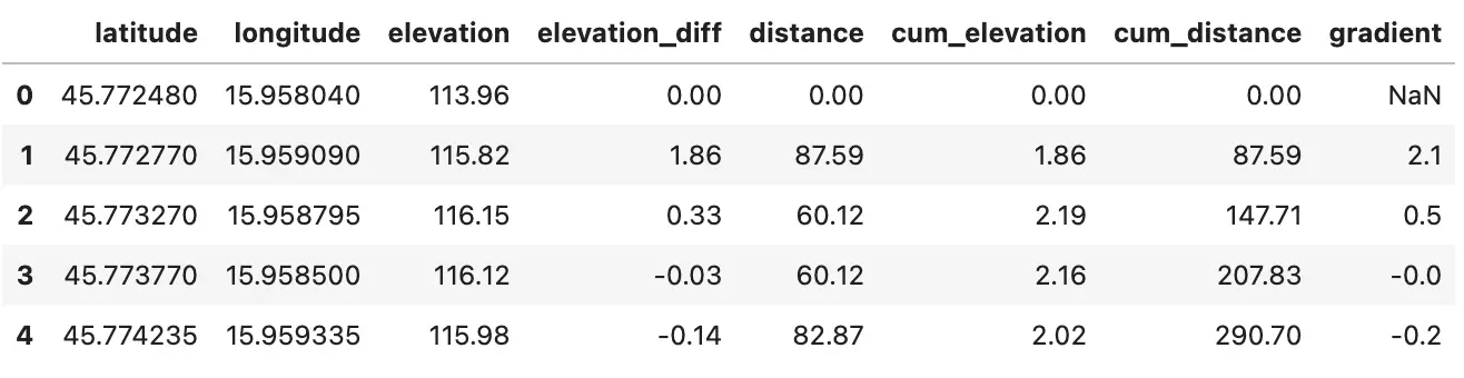
Image 5 - Route dataset with gradient info (image by author)
Let’s see where the missing values are:
route_df[route_df['gradient'].isna()]
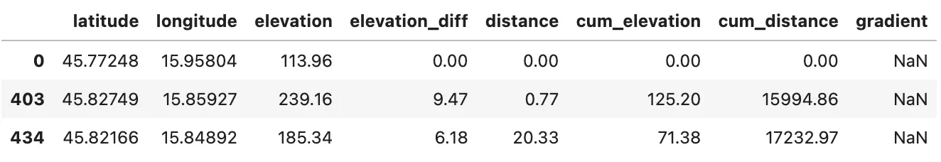
Image 6 - All missing gradient values in the dataset (image by author)
We can ignore the first one, as it’s missing for a whole different reason. We’ll have to handle the other two. To get the idea of the approach, let’s isolate the second one with the surrounding couple of rows:
route_df[401:406]
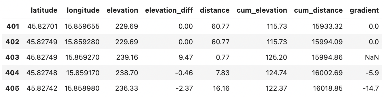
Image 7 - Data points surrounding the missing gradient value (image by author)
We’ll impute the missing values with interpolation. It will replace the missing value with the average of the data point before and after it. For example, the missing gradient before the missing value was 0, and after it was -5.9. The interpolated gradient will be -2,95, as (0 + (-5.9)) / 2 = -2.95:
route_df[401:406].interpolate()
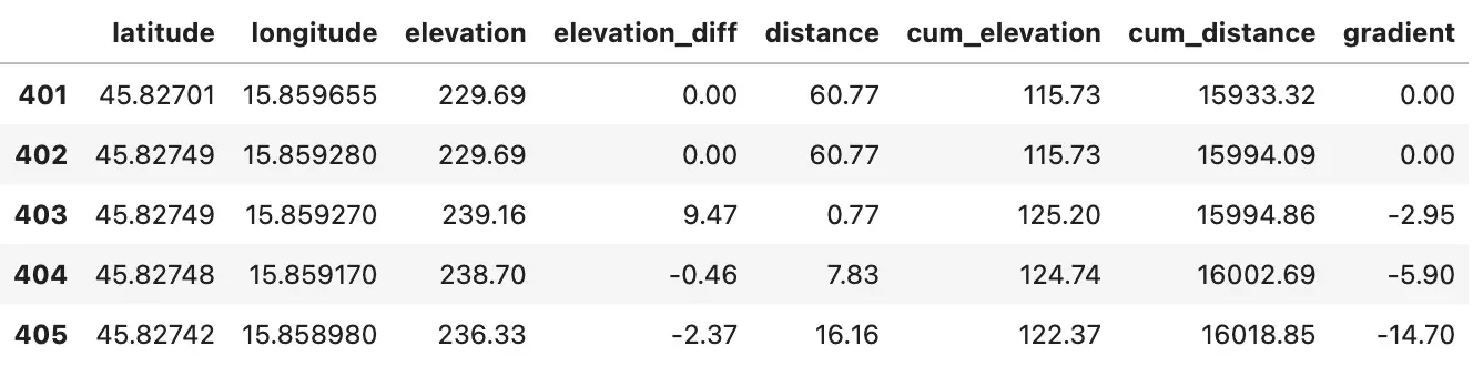
Image 8 - Interpolated gradient for a single data point (image by author)
Use the snippet below to apply interpolation to the entire dataset and fill the missing value at the first row with a zero:
route_df['gradient'] = route_df['gradient'].interpolate().fillna(0)

route_df.head()
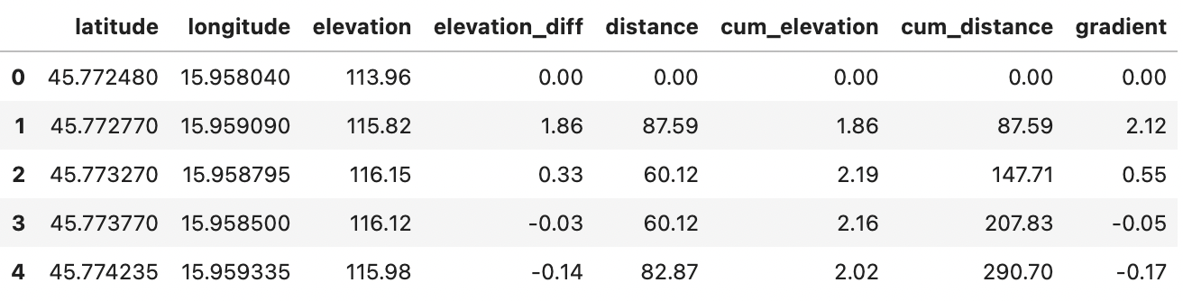
Image 9 - Dataset with interpolated gradient column
Finally, we’ll visualize the gradient to see if the line is connected this time:
plt.title('Terrain gradient on the route', size=20)
plt.xlabel('Data point', size=14)
plt.ylabel('Gradient (%)', size=14)
plt.plot(np.arange(len(route_df)), route_df['gradient'], lw=2, color='#101010');
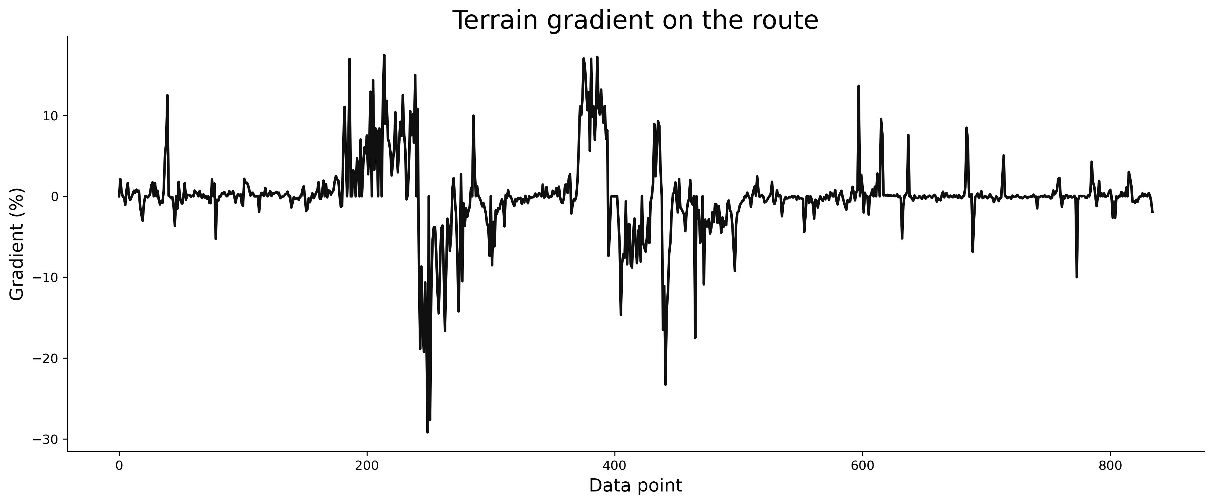
Image 10 - Estimated average route gradient v3 (image by author)
Everything looks good now, which means we’re ready to further analyze the gradient. We’ll leave that for the upcoming article, but for now please save the dataset to a CSV file:
route_df.to_csv('../data/route_df_gradient.csv', index=False)
That’s all I wanted to cover today. Let’s wrap things up next.
Conclusion
And there you have it - how to calculate and visualize gradients of a Strava route GPX file. You have to admit - it’s easier than it sounds. Everything boils to elementary school math anyone can follow. The following article will complicate things slightly, as we’ll shift our focus to gradient profiles. Put simply, we want to know the distance cycled across different gradient ranges, but don’t worry about it just yet.