Essential pillars of statistics and data science
Any data scientist can glean information from a dataset — any good data scientist will know that it takes a solid statistical underpinning to glean useful and reliable information. It’s impossible to perform quality data science without it.
But statistics is a huge field! Where do I start?
Here are the top five statistical concepts every data scientist should know: descriptive statistics, probability distributions, dimensionality reduction, over- and under-sampling, and Bayesian statistics.
Let’s start with the most simple one.
Descriptive statistics
You’re sitting in front of a dataset. How can you get a high-level description of what you’ve got? Descriptive statistics is the answer. You’ve probably heard of some of these: mean, median, mode, variance, standard deviation …
These will quickly identify key features of your dataset and inform your approach no matter the task. Let’s take a look at some of the most common descriptive stats.
Mean
The mean (also known as “expected value” or “average”) is the sum of values divided by the number of values. Take this example set:
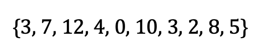
Image by author
The mean is calculated as follows:
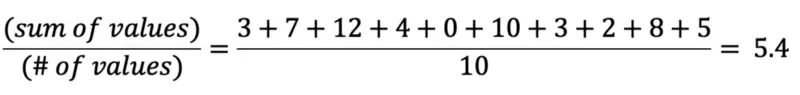
Image by author
Median
List your values in ascending (or descending) order. The median is the point that divides the data in half. If there are two middle numbers, the median is the mean of these. In our example:
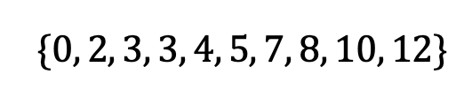
Image by author
The median is 4.5.
Mode
The mode is the most frequent value(s) in your dataset. In our example, the mode is 3.
Variance
The variance measures the spread of a dataset with respect to the mean. To calculate the variance, subtract the mean from each value. Square each difference. Finally, calculate the mean of those resulting numbers. In our example:

Image by author
Standard deviation
The standard deviation measures overall spread and is calculated by taking the square root of the variance. In our example:
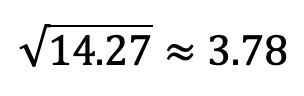
Image by author
Other descriptive statistics include skewness, kurtosis, and quartiles.
Probability distributions
A probability distribution is a function that gives the probability of occurrence for every possible outcome of an experiment. If you’re picturing a bell curve, you’re on the right track. It shows, at a glance, how the values of a random variable are dispersed. Random variables, and therefore distributions, can be either discrete or continuous.
Discrete
John is a baseball player who has a 50% random chance of hitting the ball each time it is pitched to him. Let’s throw John three pitches and see how many times he hits the ball. Here is a list of all the possible outcomes:
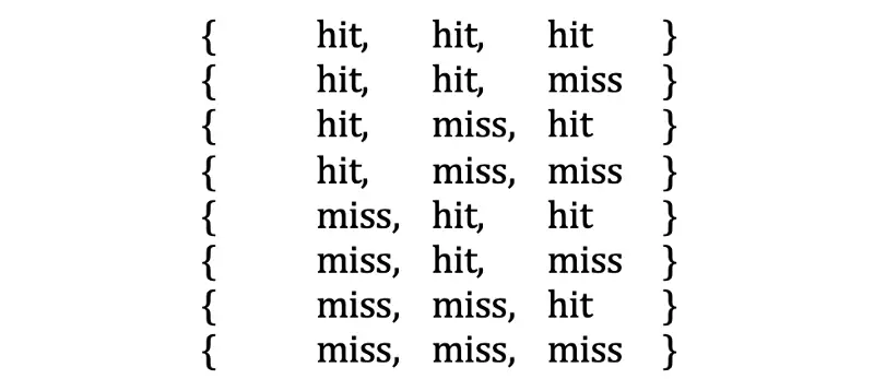
Image by author
Let X be our random variable, the number of times John gets a hit in the three-pitch experiment. The probability of John getting n hits is represented by P(X= n). So, X can be 0, 1, 2, or 3. If all eight of the above outcomes are equally likely, we have:
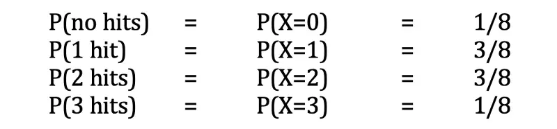
Image by author
Replace P with f and we’ve got our probability function! Let’s graph it.
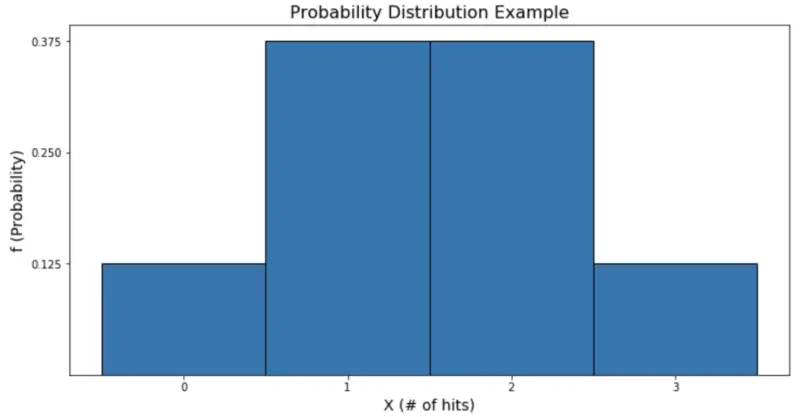
Image by author
From the graph, we see that it is more likely for John to get 1 or 2 hits than it is for him to get 0 or 3, because the graph is taller for those values of X. Common discrete distributions include Bernoulli, binomial, and Poisson.
Continuous
The continuous case follows naturally from the discrete case. Instead of counting hits, our random variable could be the time the baseball is in the air. Rather than just one, two, or three seconds, we can have values like 3.45 seconds or 6.98457 seconds.
We’re talking about a set of infinitely many possibilities. Other examples of continuous variables are height, time, and temperature. Common continuous distributions include normal, exponential, and Chi-squared.
Dimensionality reduction
If you have too many input variables or your data are computationally unwieldy, you may turn to dimensionality reduction. This is the process of projecting high-dimensional data into a lower-dimensional space, but it is important to be mindful not to lose important features of the original dataset.
For example, suppose you are trying to determine what factors best predict whether or not your favorite basketball team will win their game tonight. You may collect data such as their win percentage, who they’re playing, where they’re playing, who their starting forward is, what he ate for dinner, and what color shoe the coach is wearing.
You might suspect that certain of these features are more correlated to winning than others. Dimensionality reduction could allow us to confidently drop information that will not contribute as meaningfully to the prediction while retaining features with the most predictive value.
Principal Component Analysis (PCA) is a popular way to do this, and it works by exaggerating the variance of new combinations of features, called principal components. These new combinations are projections of the original data points into a new space — still the same dimension — where the variation is played up.
The general idea is that of these new components, those with the least variation can be most safely dropped. Dropping a single component will reduce the original dimensionality by one, dropping two components will reduce it by two, and so on.
Under-sampling and Over-sampling
A collective set of observations is called the “sample”, and the way that the set was collected is called “sampling”. In a classification situation where you need minority and majority classes to be equally represented, under- or over-sampling may be useful. Under-sampling the majority class or over-sampling the minority class can help even out an unbalanced dataset.
Random over-sampling (alternatively, random under-sampling) involves randomly selecting and duplicating observations in the minority class (or randomly selecting and deleting observations in the majority class).
This is easy to implement, but you should proceed with caution: over-sampling weights the observations that are duplicated, which can heavily influence results if they were not unbiased, to begin with. Similarly, under-sampling runs the risk of deleting key observations.
One way to over-sample the minority class is the Synthetic Minority Over-sampling Technique (SMOTE). This creates (synthetic) minority class observations by creating new combinations of existing observations. For each observation in the minority class, _SMOTE_calculates its k nearest neighbors; that is, it finds the k minority class observations that are most like the observation.
Viewing observations as vectors, it creates random linear combinations by weighting any of the k nearest neighbors by a random number between 0 and 1 and adding it to the original vector.
One way to under-sample of the majority class is with cluster centroids. Similar in theory to SMOTE, it replaces groups of vectors by the centroid of their k nearest neighbors cluster.
Bayesian statistics
When it comes to statistical inference, there are two main schools of thought: frequentist statistics and Bayesian statistics. Frequentist statistics allows us to do meaningful work, but there are cases where it falls short. Bayesian statistics does well when you have reason to believe that your data may not be a good representation of what you expect to observe in the future.
This allows you to incorporate your own knowledge into your calculations, rather than solely relying on your sample. It also allows you to update your thoughts about the future after new data come in.
Consider an example: Team A and Team B have played each other 10 times, and Team A has won 9 of those times. If the teams are playing each other tonight, and I ask you who you think will win, you’d probably say Team A! What if I also told you that Team B has bribed tonight’s referees? Well, then you might guess that Team B will win.
Bayesian statistics allows you to incorporate this extra information into your calculations, while frequentist statistics focuses solely on the 9 out of 10 win percentage.
Bayes’ Theorem is the key:
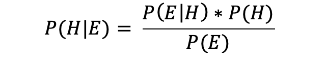
Image by author
The conditional probability of H given E, written P( H| E), represents the probability of H occurring given that E also occurs (or has occurred). In our example, H is the hypothesis that Team B will win, and E is the evidence that I gave you about Team B bribing the referees.
P( H) is the frequentist probability, 10%. P( E| H) is the probability that what I told you about the bribe is true, given that Team B wins. (If Team B wins tonight, would you believe what I told you?)
Finally, P( E) is the probability that Team B has in fact bribed the referees. Am I a trustworthy source of information? You can see that this approach incorporates more information than just the outcomes of the two teams’ previous 10 match-ups.
And that’s it for today. Let’s wrap things up in the next section.
Before you go
Learning these 5 concepts won’t make you a master of statistics or data science — but it is a great place to start if you can’t understand the basic flow of a data science project.
If it still sounds like something advanced, my recommendation is to start small. Here’s the best introductory statistics book voted by me and many others:
The Single Best Introductory Statistics Book for Data Science
And we’re done — thanks for reading.