
From data gathering and preparation to model training and evaluation — Source code included.
Deep learning is kind of a big deal these days. Heck, it’s even a requirement for most data science jobs, even entry-level ones. There’s no better introductory lecture than regression. You already know the concepts from basic statistics and machine learning, and now it’s time to bring neural networks into the mix.
This article will show you how. By the end, you’ll have a fully functional model for predicting housing prices which you can attach to your portfolio — after some modifications, preferred.
Don’t feel like reading? Watch my video instead:
You can download the source code on GitHub.
Dataset used
Let’s keep things simple today and stick with a well-known Housing prices dataset:
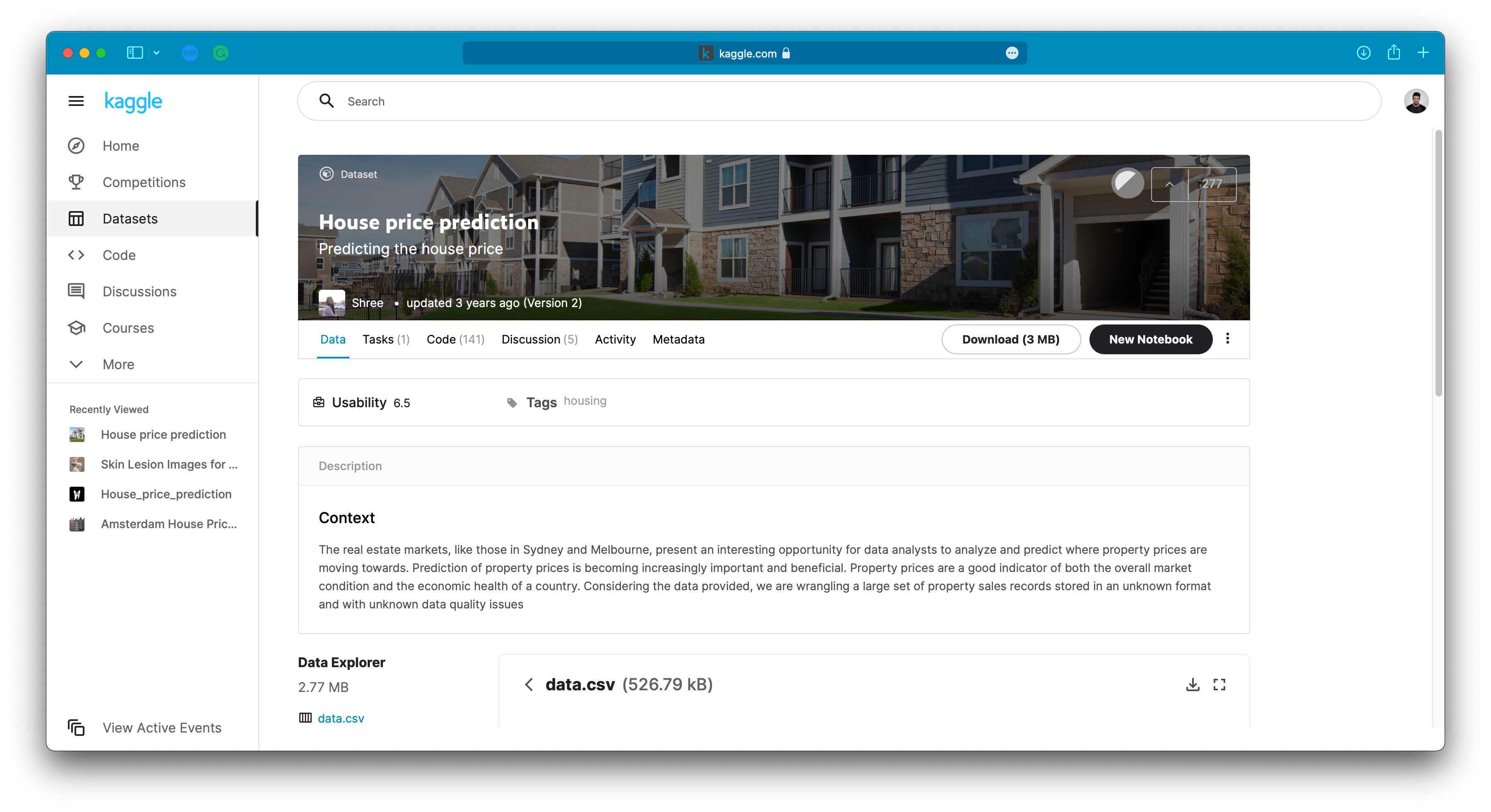
Image 1 — Housing prices dataset from Kaggle (image by author)
It has a bunch of features that are initially unusable with the neural network model, so you’ll have to spend some time dealing with them. Download the dataset, extract the ZIP file, and place the CSV dataset somewhere safe.
Then activate the virtual environment that has TensorFlow 2+ installed and launch JupyterLab. You’re free to use any other IDE, but all the screenshots below will be from Jupyter.
Dataset exploration and preparation
The first step is to import Numpy and Pandas, and then to import the dataset. The following snippet does that and also prints a random couple of rows:
import numpy as np
import pandas as pd

df = pd.read_csv('data/data.csv')
df.sample(5)
Here’s how the dataset looks like:
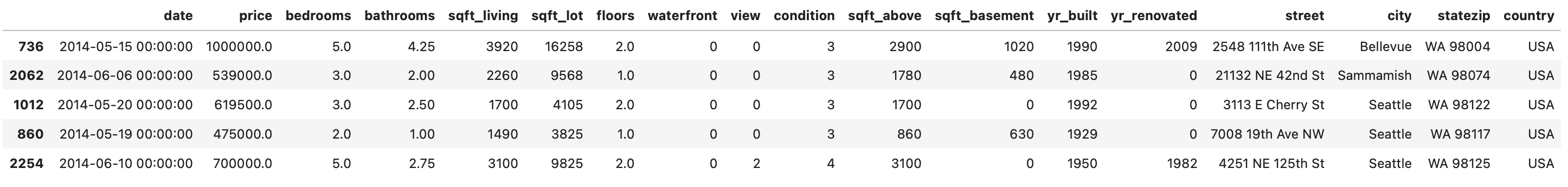
Image 2 — Housing prices dataset (image by author)
You definitely can’t pass it to a neural network in this format.
Deleting unnecessary columns
Since we want to avoid spending too much time preparing the data, it’s best to drop most of the non-numeric features. Keep only the city column, as it’s simple enough to encode:
to_drop = ['date', 'street', 'statezip', 'country']
df = df.drop(to_drop, axis=1)

df.head()
Here’s how it should look like now:
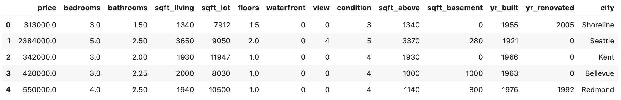
Image 3 — Dataset after removing most of the string columns (image by author)
You definitely could keep all columns and do some feature engineering with them. It would likely increase the performance of the model. But even this will be enough for what you need today.
Feature engineering
Now you’ll spend some time tweaking the dataset. The yr_renovated column sometimes has the value of 0. I assume that’s because the house wasn’t renovated. You’ll create a couple of features — house age, was the house renovated or not, was it renovated in the last 10 years, and was it renovated in the last 30 years.
You can use list comprehension for every mentioned feature. Here’s how:
# How old is the house?
df['house_age'] = [2021 - yr_built for yr_built in df['yr_built']]

# Was the house renovated and was the renovation recent?
df['was_renovated'] = [1 if yr_renovated != 0 else 0
    for yr_renovated in df['yr_renovated']]
df['was_renovated_10_yrs'] = [1 if (2021 - yr_renovated) <= 10
    else 0 for yr_renovated in df['yr_renovated']]
df['was_renovated_30_yrs'] = [1 if 10 < (2021 - yr_renovated) <= 30
    else 0 for yr_renovated in df['yr_renovated']]

# Drop original columns
df = df.drop(['yr_built', 'yr_renovated'], axis=1)
df.head()
Here’s how the dataset looks now:
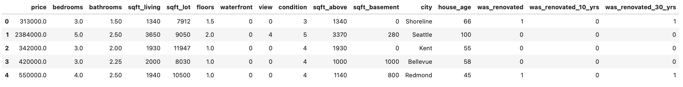
Image 4 — Dataset after feature engineering (1) (image by author)
Let’s handle the city column next. Many cities have only a couple of houses listed, so you can declare a function that will get rid of all city values that don’t occur often. That’s what the remap_location() function will do — if there are less than 50 houses in that city, it’s replaced with something else. It’s just a way to reduce the number of options:
def remap_location(data: pd.DataFrame,
                   location: str,
                   threshold: int = 50) -> str:
    if len(data[data['city'] == location]) < threshold:
        return 'Rare'
    return location
Let’s test the function — the city of Seattle has many houses listed, while Fall City has only 11:
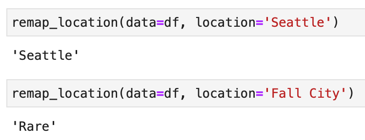
Image 5 — Remapping city values (image by author)
Let’s apply this function to all cities and print a sample of 10 rows:
df['city'] = df['city'].apply(
    lambda x: remap_location(data=df, location=x)
)
df.sample(10)
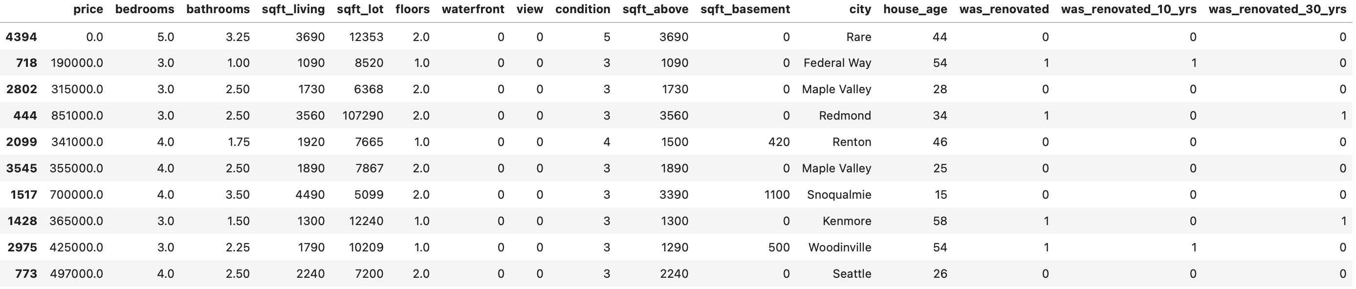
Image 6 — Dataset after feature engineering (2) (image by author)
Everything looks as it should, so let’s continue.
Target variable visualization
Anytime you’re dealing with prices, it’s unlikely the target variable will be distributed normally. And this housing dataset is no exception. Let’s verify it by importing Matplotlib and visualizing the distribution with a Histogram:
import matplotlib.pyplot as plt
from matplotlib import rcParams
rcParams['figure.figsize'] = (16, 6)
rcParams['axes.spines.top'] = False
rcParams['axes.spines.right'] = False

plt.hist(df['price'], bins=100);
Here’s how it looks like:
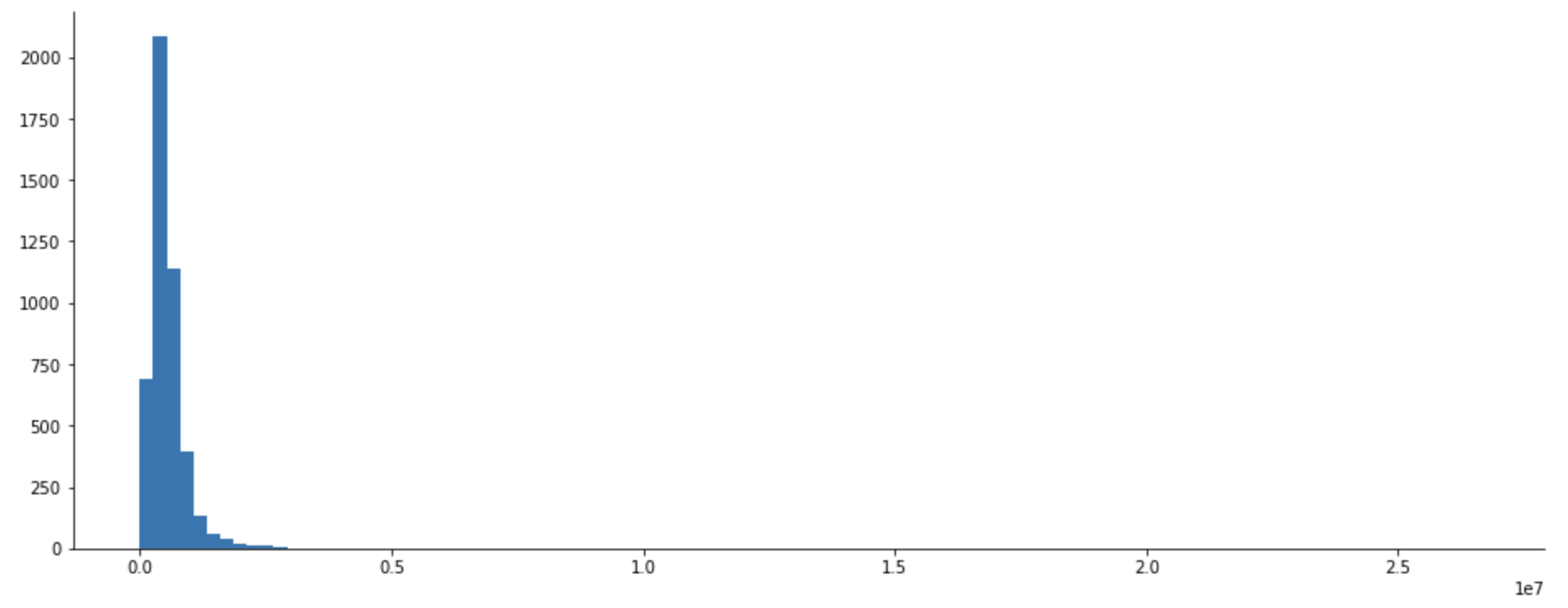
Image 7 — Target variable histogram (1) (image by author)
Outliers are definitely present, so let’s handle them next. The pretty common thing to do is to calculate Z-scores. They let you know how many standard deviations a value is located from the mean. In the case of a normal distribution, anything below or above 3 standard deviations is classified as an outlier. The distribution of prices isn’t normal, but let’s still do the Z-test to remove the houses on the far right.
You can calculate the Z-score with Scipy. You’ll assign them as a new dataset column —price_z, and then keep only the rows in which the absolute value of Z is less than or equal to three.
There are also around 50 houses listed for $0, so you’ll delete those as well:
from scipy import stats


# Calculate Z-values
df['price_z'] = np.abs(stats.zscore(df['price']))

# Filter out outliers
df = df[df['price_z'] <= 3]

# Remove houses listed for $0
df = df[df['price'] != 0]

# Drop the column
df = df.drop('price_z', axis=1)

# Draw a histogram
plt.hist(df['price'], bins=100);
Here’s how the distribution looks like now:

Image 8 — Target variable histogram (2) (image by author)
There’s still a bit of skew present, but let’s declare it good enough.
As the last step, let’s convert the data into a format ready for machine learning.
Data preparation for ML
A neural network likes to see only numerical data on the same scale. Our dataset isn’t, and we also have some non-numerical data. That’s where data scaling and one-hot encoding come into play.
You could now transform each feature individually, but there’s a better way. You can use the make_column_transformer() function from Scikit-Learn to apply scaling and encoding in one go.
You can ignore features like waterfront, was_renovated, was_renovated_10_yrs, and was_renovated_30_yrs, as they already are in the format you need:
from sklearn.compose import make_column_transformer
from sklearn.preprocessing import MinMaxScaler, OneHotEncoder


transformer = make_column_transformer(
    (MinMaxScaler(),
        ['sqft_living', 'sqft_lot','sqft_above',
         'sqft_basement', 'house_age']),
    (OneHotEncoder(handle_unknown='ignore'),
        ['bedrooms', 'bathrooms', 'floors',
         'view', 'condition'])
)
Next, let’s separate features from the target variable, and split the dataset into training and testing parts. The train set will account for 80% of the data, and we’ll use everything else for testing:
from sklearn.model_selection import train_test_split


X = df.drop('price', axis=1)
y = df['price']

X_train, X_test, y_train, y_test = train_test_split(
    X, y, test_size=0.2, random_state=42
)
And finally, you can apply the transformations declared a minute ago. You’ll fit and transform the training features, and only apply the transformations to the testing set:
# Fit
transformer.fit(X_train)

# Apply the transformation
X_train = transformer.transform(X_train)
X_test = transformer.transform(X_test)
You won’t be able to inspect X_train and X_test directly, as they’re now stored as a sparse matrix:

Image 9 — Sparse matrix (image by author)
TensorFlow won’t be able to read that format, so you’ll have to convert it to a multidimensional Numpy array. You can use the toarray() function. Here’s an example:
X_train.toarray()
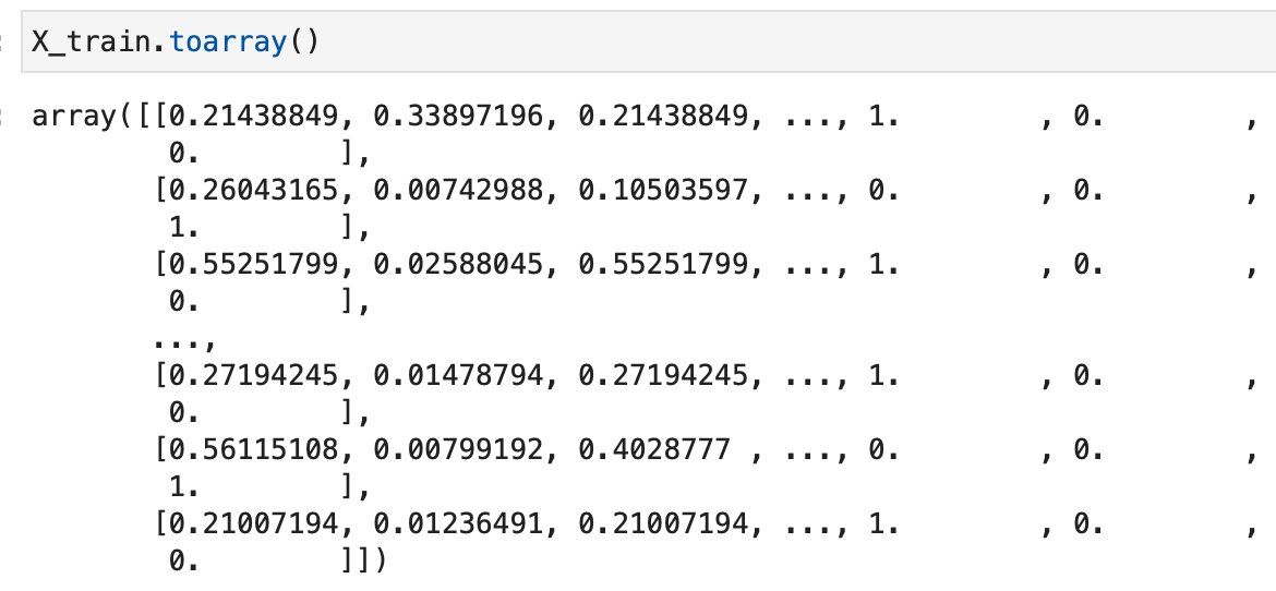
Image 10 — Sparse matrix to Numpy array (image by author)
Convert both feature sets to a Numpy array, and you’re good to go:
X_train = X_train.toarray()
X_test = X_test.toarray()
Let’s finally train the model.
Training a regression model with TensorFlow
You’ll now build a sequential model made of fully connected layers. There are many imports to do, so let’s get that out of the way:
import tensorflow as tf
from tensorflow.keras import Sequential
from tensorflow.keras.layers import Dense
from tensorflow.keras.optimizers import Adam
from tensorflow.keras import backend as K
Loss tracking
You’re dealing with housing prices here, so the loss could be quite huge if you track it through, let’s say, mean squared error. That metric also isn’t very useful to you, as it basically tells you how wrong your model is in units squared.
You can calculate the square root of the MSE to go back to the original units. That metric isn’t supported by default, but we can declare it manually. Keep in mind that you’ll have to use functions from Keras backend to make it work:
def rmse(y_true, y_pred):
    return K.sqrt(K.mean(K.square(y_pred - y_true)))
Building a model
And now you can finally declare a model. It will be a simple one, having just three hidden layers of 256, 256, and 128 units. Feel free to experiment with these, as there’s no right or wrong way to set up a neural network. These layers are then followed by an output layer of one node, since you’re predicting a numerical value.
You’ll then compile a model using the RMSE as a way to keep track of the loss and as an evaluation metric, and you’ll optimize the model using the Adam optimizer.
Finally, you’ll train the model on the training data for 100 epochs:
tf.random.set_seed(42)

model = Sequential([
    Dense(256, activation='relu'),
    Dense(256, activation='relu'),
    Dense(128, activation='relu'),
    Dense(1)
])

model.compile(
    loss=rmse,
    optimizer=Adam(),
    metrics=[rmse]
)

model.fit(X_train, y_train, epochs=100)
The training should finish in a minute or so, depending on the hardware behind:
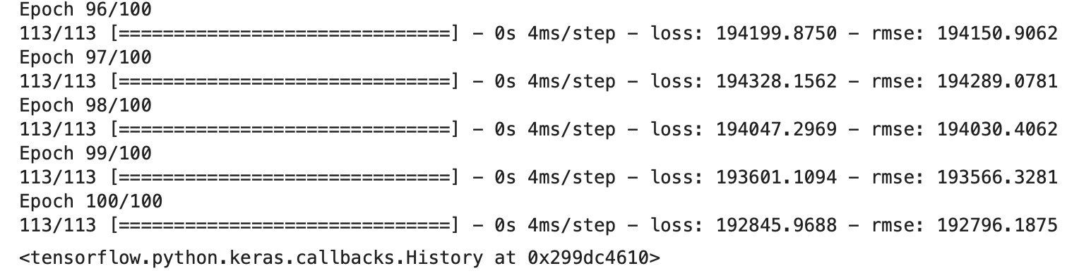
Image 11 — Regression model training with TensorFlow (image by author)
The final RMSE value on the training set is just above 192000, which means that for an average house, the model is wrong in the price estimate by $192000.
Making predictions
You can make predictions on the test set:
predictions = model.predict(X_test)
predictions[:5]
Here’s how the first five predictions look like:
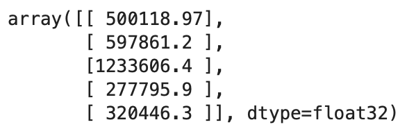
Image 12 — First 5 predictions (image by author)
You’ll have to convert these to a 1-dimensional array if you want to calculate any metrics. You can use the ravel() function from Numpy to do so:
predictions = np.ravel(predictions)
predictions[:5]
Here are the results:

Image 13 — First 5 predictions as a 1D array (image by author)
Model evaluation
And now let’s evaluate the predictions on the test set by using RMSE:
rmse(y_test, predictions).numpy()
You’ll get 191000 as an error value, which indicates the model hasn’t overfitted on the training data. You’d likely get better results with a more complex model training for more epochs. That’s something you can experiment with on your own.
Parting words
And that does it — you’ve trained a simple neural network model by now, and you know how to make predictions on the new data. Still, there’s a lot you could improve.
For example, you could spend much more time preparing the data. We deleted the date-time feature, the street information, the zip code and so on, which could be valuable for the model performance. The thing is — those would take too much time to prepare, and I want to keep these articles somewhat short.
You could also add additional layers to the network, increase the number of neurons, choose different activation functions, select a different optimizer, add dropout layers, and much more. The possibilities are almost endless, so it all boils down to experimentation.
The following article will cover how to build a classification model using TensorFlow, so stay tuned if you want to learn more.
Thanks for reading.
Stay connected
- Sign up for my newsletter
- Subscribe on YouTube
- Connect on LinkedIn