
Let’s develop a real-time web scraping application with R — way easier than with Python
A good dataset is difficult to find. That’s expected, but nothing to fear about. Techniques like web scraping enable us to fetch data from anywhere at any time — if you know how. Today we’ll explore just how easy it is to scrape web data with R and do so through R Shiny’s nice GUI interface.
So, what is web scraping? In a nutshell, it’s just a technique of gathering data from various websites. One might use it when:
- There’s no dataset available for the needed analysis
- There’s no public API available
Still, you should always check the site’s policy on web scraping, alongside with this article on Ethics in web scraping. After that, you should be able to use common sense to decide if scraping is worth it.
If it feels wrong, don’t do it.
Luckily, some websites are made entirely for practicing web scraping. One of them is books.toscrape.com, which, as the name suggests, lists made up books in various genres:
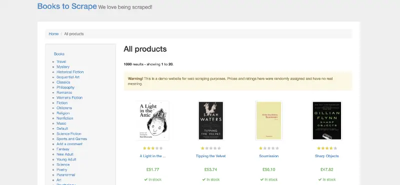
Screenshot from http://books.toscrape.com
So, let’s scrape the bastard next, shall we?
Plan of attack
Open up the webpage and click on any two categories (sidebar on the left), and inspect the URL. Here’s our pick:
http://books.toscrape.com/catalogue/category/books/<strong>travel_2</strong>/index.htmlhttp://books.toscrape.com/catalogue/category/books/<strong>mystery_3</strong>/index.html
What do these URLs have in common? Well, everything except for the bolded part. That’s the category itself. No idea what’s the deal with the numbering, but it is what it is. Every page contains a list of books, and a single book looks like this:
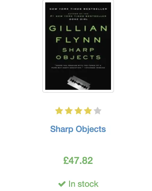
Screenshot of a single book in Mystery category
Our job is to grab the information for every book in a category. Doing this requires a bit of HTML knowledge, but it’s a simple markup language, so I don’t see a problem there.
We want to scrape:
- Title —h3 > a > title property
- Rating —p.star-rating > class attribute
- Price —div.product_price > div.price_color > text
- Availability —div.product_price > div.instock > text
- Book URL —div.image_container > a > href property
- Thumbnail URL —div.image_container > img > src property
You know everything now, so let’s start with the scraping next.
Scraping books
The rvest package is used in R to perform web scraping tasks. It’s very similar to dplyr, a well-known data analysis package, due to the pipe operator’s usage and the behavior in general. We know how to get to certain elements, but how to implement this logic in R?
Here’s an example of how to scrape book titles in the travel category:
library(rvest)

url <- 'http://books.toscrape.com/catalogue/category/books/travel_2/index.html'
titles <- read_html(url) %>%
  html_nodes('h3') %>%
  html_nodes('a') %>%
  html_text()
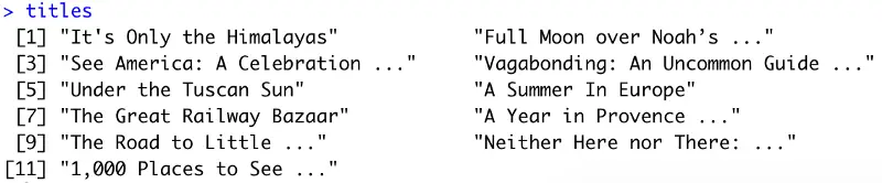
Image by author
Wasn’t that easy? We can similarly scrape everything else. Here’s the script:
library(rvest)
library(stringr)

titles <- read_html(url) %>%
  html_nodes('h3') %>%
  html_nodes('a') %>%
  html_text()

urls <- read_html(url) %>%
  html_nodes('.image_container') %>%
  html_nodes('a') %>%
  html_attr('href') %>%
  str_replace_all('../../../', '/')

imgs <- read_html(url) %>%
  html_nodes('.image_container') %>%
  html_nodes('img') %>%
  html_attr('src') %>%
  str_replace_all('../../../../', '/')

ratings <- read_html(url) %>%
  html_nodes('p.star-rating') %>%
  html_attr('class') %>%
  str_replace_all('star-rating ', '')

prices <- read_html(url) %>%
  html_nodes('.product_price') %>%
  html_nodes('.price_color') %>%
  html_text()

availability <- read_html(url) %>%
  html_nodes('.product_price') %>%
  html_nodes('.instock') %>%
  html_text() %>%
  str_trim()
Awesome! As a final step, let’s glue all of this together in a single Data frame:
scraped <- data.frame(
  Title = titles,
  URL = urls,
  SourceImage = imgs,
  Rating = ratings,
  Price = prices,
  Availability = availability
)
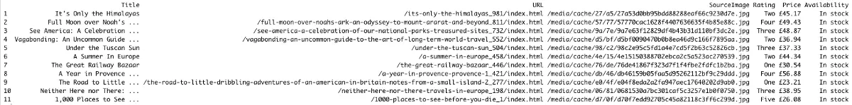
Image by author
You can end the article here and call it a day, but there’s something else we can build from this — a simple, easy to use web application. Let’s do that next.
Web application for scraping
R has a fantastic library for web/dashboard development —Shiny. It’s far easier to use than anything similar in Python, so we’ll stick with it. To start, create a new R file and paste the following code inside:
library(shiny)
library(rvest)
library(stringr)
library(glue)

ui <- fluidPage()

server <- function(input, output) {}

shinyApp(ui=ui, server=server)
It is a boilerplate every Shiny app requires. Next, let’s style the UI. We’ll need:
- Title — just a big, bold text on top of everything (optional)
- Sidebar — contains a dropdown menu to select a book genre
- Central area — displays a table output once the data gets scraped
Here’s the code:
ui <- fluidPage(
  column(12, tags$h2('Real-time web scraper with R')),
  sidebarPanel(
    width=3,
    selectInput(
      inputId='genreSelect',
      label='Genre',
      choices=c('Business', 'Classics', 'Fiction', 'Horror', 'Music'),
      selected='Business',
    )
  ),
  mainPanel(
    width=9,
    tableOutput('table')
  )
)
Next, we need to configure the server function. It has to remap our nicely formatted inputs to an URL portion (e.g., ‘Business’ to ‘business_35’) and scrape data for the selected genre. We already know how to do so. Here’s the code for the server function:
server <- function(input, output) {
  output$table <- renderTable({
    mappings <- c('Business' = 'business_35', 'Classics' = 'classics_6', 'Fiction' = 'fiction_10',
                  'Horror' = 'horror_31', 'Music' = 'music_14')

    url <- glue('http://books.toscrape.com/catalogue/category/books/', mappings[input$genreSelect], '/index.html')

    titles <- read_html(url) %>%
      html_nodes('h3') %>%
      html_nodes('a') %>%
      html_text()

    urls <- read_html(url) %>%
      html_nodes('.image_container') %>%
      html_nodes('a') %>%
      html_attr('href') %>%
      str_replace_all('../../../', '/')

    imgs <- read_html(url) %>%
      html_nodes('.image_container') %>%
      html_nodes('img') %>%
      html_attr('src') %>%
      str_replace_all('../../../../', '/')

    ratings <- read_html(url) %>%
      html_nodes('p.star-rating') %>%
      html_attr('class') %>%
      str_replace_all('star-rating ', '')

    prices <- read_html(url) %>%
      html_nodes('.product_price') %>%
      html_nodes('.price_color') %>%
      html_text()

    availability <- read_html(url) %>%
      html_nodes('.product_price') %>%
      html_nodes('.instock') %>%
      html_text() %>%
      str_trim()

    data.frame(
      Title = titles,
      URL = urls,
      SourceImage = imgs,
      Rating = ratings,
      Price = prices,
      Availability = availability
    )
  })
}
And that’s it — we can run the app now and inspect the behavior!

GIF by author
Just what we wanted — simple, but still entirely understandable. Let’s wrap things up in the next section.
Parting words
In only a couple of minutes, we went from zero to a working web scraping application. Options to scale this are endless — add more categories, work on the visuals, include more data, format data more nicely, add filters, etc.
I hope you’ve managed to follow and that you’re able to see the power of web scraping. This was a dummy website and a dummy example, but the approach stays the same irrelevant to the data source.
Thanks for reading.