No dataset? No problem. Create your own in seconds with Python.
A good dataset is difficult to find. Besides, sometimes you just want to make a point. Tedious loadings and preparations can be a bit much for these cases.
Today you’ll learn how to make synthetic datasets with Python and Scikit-Learn — a fantastic machine learning library. You’ll also learn how to play around with noise, class balance, and class separation.
You can download the Notebook for this article here.
Make your first synthetic dataset
Real-world datasets are often too much for demonstrating concepts and ideas. Imagine you want to visually explain SMOTE (a technique for handling class imbalance). You first have to find a class-imbalanced dataset and project it to 2–3 dimensions for visualizations to work.
There’s a better way.
The Scikit-Learn library comes with a handy make_classification() function. It’s not the only one for creating synthetical datasets, but you’ll use it heavily today. It accepts various parameters that let you control the looks and feels of the dataset, but more on that in a bit.
To start, you’ll need to import the required libraries. Refer to the following snippet:
import numpy as np
import pandas as pd
from sklearn.datasets import make_classification

import matplotlib.pyplot as plt
from matplotlib import rcParams
rcParams['axes.spines.top'] = False
rcParams['axes.spines.right'] = False
You’re ready to create your first dataset. It’ll have 1000 samples assigned to two classes (0 and 1) with a perfect balance (50:50). All samples belonging to each class are centered around a single cluster. The dataset has only two features — to make the visualization easier:
X, y = make_classification(
    n_samples=1000,
    n_features=2,
    n_redundant=0,
    n_clusters_per_class=1,
    random_state=42
)

df = pd.concat([pd.DataFrame(X), pd.Series(y)], axis=1)
df.columns = ['x1', 'x2', 'y']
# 5 random rows
df.sample(5)
A call to sample() prints out five random data points:
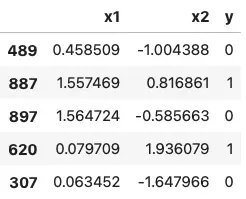
Image 1 — Random sample of 5 rows (image by author)
This doesn’t give you the full picture behind the dataset. It’s two dimensional, so you can declare a function for data visualization. Here’s one you can use:
def plot(df: pd.DataFrame, x1: str, x2: str, y: str, title: str = '', save: bool = False, figname='figure.png'):
    plt.figure(figsize=(14, 7))
    plt.scatter(x=df[df[y] == 0][x1], y=df[df[y] == 0][x2], label='y = 0')
    plt.scatter(x=df[df[y] == 1][x1], y=df[df[y] == 1][x2], label='y = 1')
    plt.title(title, fontsize=20)
    plt.legend()
    if save:
        plt.savefig(figname, dpi=300, bbox_inches='tight', pad_inches=0)
    plt.show()


plot(df=df, x1='x1', x2='x2', y='y', title='Dataset with 2 classes')
Here’s how it looks like visually:
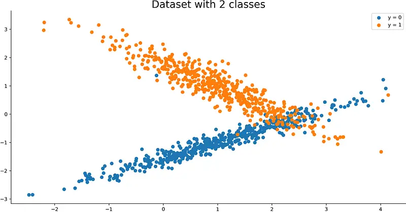
Image 2 — Visualization of a synthetic dataset (image by author)
That was fast! You now have a simple synthetic dataset you can play around with. Next, you’ll learn how to add a bit of noise.
Add noise
You can use the flip_y parameter of the make_classification() function to add noise.
This parameter represents the fraction of samples whose class is assigned randomly. Larger values introduce noise in the labels and make the classification task harder. Note that the default setting flip_y > 0 might lead to less than n_classes in y in some cases[1].
Here’s how to use it with our dataset:
X, y = make_classification(
    n_samples=1000,
    n_features=2,
    n_redundant=0,
    n_clusters_per_class=1,
    flip_y=0.15,
    random_state=42
)

df = pd.concat([pd.DataFrame(X), pd.Series(y)], axis=1)
df.columns = ['x1', 'x2', 'y']

plot(df=df, x1='x1', x2='x2', y='y', title='Dataset with 2 classes - Added noise')
Here’s the corresponding visualization:
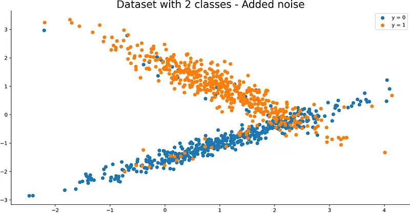
Image 3 — Visualization of a synthetic dataset with added noise (image by author)
You can see many more orange points in the blue cluster and vice versa, at least when compared with Image 2.
That’s how you can add noise. Let’s shift the focus on class balance next.
Tweak class balance
It’s common to see at least a bit of class imbalance in the real-world datasets. Some datasets suffer from severe class imbalance. For example, one of 1000 bank transactions could be fraudulent. This means the balance ratio is 1:1000.
You can use the weights parameter to control class balance. It excepts a list as a value with N – 1 values, where N is the number of features. We only have 2, so there’ll be a single value in the list.
Let’s see what happens if we specify 0.95 as a value:
X, y = make_classification(
    n_samples=1000,
    n_features=2,
    n_redundant=0,
    n_clusters_per_class=1,
    weights=[0.95],
    random_state=42
)

df = pd.concat([pd.DataFrame(X), pd.Series(y)], axis=1)
df.columns = ['x1', 'x2', 'y']

plot(df=df, x1='x1', x2='x2', y='y', title='Dataset with 2 classes - Class imbalance (y = 1)')
Here’s how the dataset looks like visually:
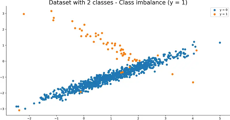
Image 4 — Visualization of a synthetic dataset with a class imbalance on positive class (image by author)
As you can see, only 5% of the dataset belongs to class 1. You can turn this around easily. Let’s say you want 5% of the dataset in class 0:
X, y = make_classification(
    n_samples=1000,
    n_features=2,
    n_redundant=0,
    n_clusters_per_class=1,
    weights=[0.05],
    random_state=42
)

df = pd.concat([pd.DataFrame(X), pd.Series(y)], axis=1)
df.columns = ['x1', 'x2', 'y']

plot(df=df, x1='x1', x2='x2', y='y', title='Dataset with 2 classes - Class imbalance (y = 0)')
Here’s the corresponding visualization:
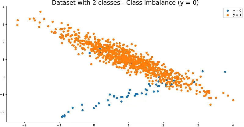
Image 5 — Visualization of a synthetic dataset with a class imbalance on negative class (image by author)
And that’s all there is to class balance. Let’s finish by tweaking class separation.
Tweak class separation
By default, there are some overlapping data points (class 0 and class 1). You can use the class_sep parameter to control how separated the classes are. The default value is 1.
Let’s see what happens if you set the value to 5:
X, y = make_classification(
    n_samples=1000,
    n_features=2,
    n_redundant=0,
    n_clusters_per_class=1,
    class_sep=5,
    random_state=42
)

df = pd.concat([pd.DataFrame(X), pd.Series(y)], axis=1)
df.columns = ['x1', 'x2', 'y']

plot(df=df, x1='x1', x2='x2', y='y', title='Dataset with 2 classes - Make classification easier')
Here’s how the dataset looks like:
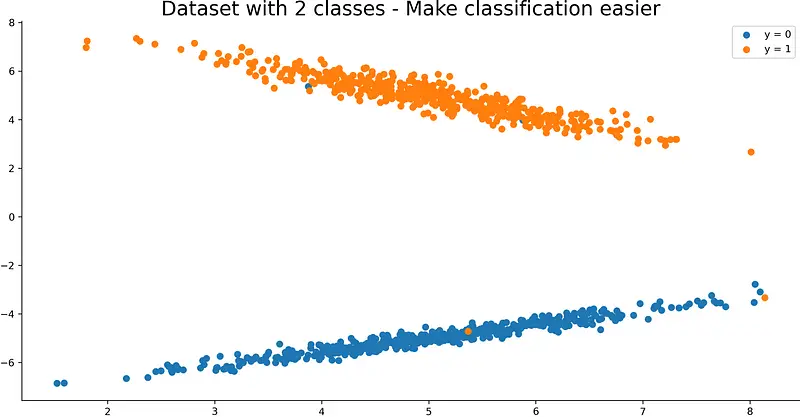
Image 6 — Visualization of a synthetic dataset with a severe class separation (image by author)
As you can see, the classes are much more separated now. Higher parameter values result in better class separation, and vice versa.
You now know everything to make basic synthetic datasets for classification. Let’s wrap things up next.
Conclusion
Today you’ve learned how to make basic synthetic classification datasets with Python and Scikit-Learn. You can use them whenever you want to prove a point or implement some data science concept. Real datasets can be overkill for that purpose, as they often require rigorous preparation.
Feel free to explore official documentation to learn about other useful parameters.
[1] https://scikit-learn.org/stable/modules/generated/sklearn.datasets.make_classification.html
Learn More
- Python If-Else Statement in One Line - Ternary Operator Explained
- Python Structural Pattern Matching - Top 3 Use Cases to Get You Started
- Dask Delayed - How to Parallelize Your Python Code With Ease
Stay connected
- Sign up for my newsletter
- Subscribe on YouTube
- Connect on LinkedIn

