Solving classification tasks with PyCaret — it’s easier than you think.
A few days back I’ve covered the basics of the PyCaret library, and also how to use it to handle regression tasks. If you are new here, PyCaret is a low-code machine learning library that does everything for you — from model selection to deployment. Reading the previous two articles isn’t a prerequisite, but feel free to go through them if you haven’t used the library before.
Classification problems are the most common type of machine learning problems — is message spam or not, will the customer leave, is the test result positive or negative — to state a few examples. For that reason, we need to know how to handle classification tasks, and how to do so with ease.
For developers, PyCaret is considered to be better and more friendly than Scikit-Learn. Both are great, don’t get me wrong, but PyCaret will save you so much time that would otherwise be spent on model selection and fine-tuning. And that’s the least fun part of the job.
This article assumes you’re familiar with the concept of classification in machine learning. You don’t have to be an expert, but its assumed you know how to fit a model to data in other libraries.
The article is structured as follows:
- Dataset overview and cleaning
- Model selection and training
- Model visualization and interpretation
- Predictions and saving the model
- Conclusion
Without much ado, let’s get started!
Dataset overview and cleaning
In most of my classification-based articles, I like to go with the Titanic dataset. There are multiple reasons why, the most obvious one being that it is fairly simple, but not too simple with regards to data cleaning and preparation.
We can load it in Pandas directly from GitHub:
data = pd.read_csv('https://raw.githubusercontent.com/datasciencedojo/datasets/master/titanic.csv')
data.head()
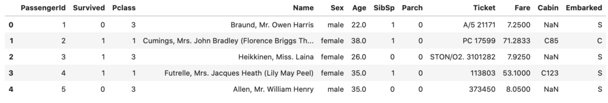
Image by author
Now we can proceed with the data cleaning itself. Here’s what I want to do:
- Drop irrelevant columns (Ticket and PassengerId)
- Remap Sex column to zeros and ones
- Check if a passenger had a unique title (like doctor) or had something more generic (like Mr., Miss.) — can be extracted from the Name column
- Check if cabin information was known — if the value of Cabin column is not NaN
- Create dummy variables from the Embarked column — 3 options
- Fill Age values with the simple mean
And here’s the code:
data.drop(['Ticket', 'PassengerId'], axis=1, inplace=True)

gender_mapper = {'male': 0, 'female': 1}
data['Sex'].replace(gender_mapper, inplace=True)

data['Title'] = data['Name'].apply(lambda x: x.split(',')[1].strip().split(' ')[0])
data['Title'] = [0 if x in ['Mr.', 'Miss.', 'Mrs.'] else 1 for x in data['Title']]
data = data.rename(columns={'Title': 'Title_Unusual'})
data.drop('Name', axis=1, inplace=True)

data['Cabin_Known'] = [0 if str(x) == 'nan' else 1 for x in data['Cabin']]
data.drop('Cabin', axis=1, inplace=True)

emb_dummies = pd.get_dummies(data['Embarked'], drop_first=True, prefix='Embarked')
data = pd.concat([data, emb_dummies], axis=1)
data.drop('Embarked', axis=1, inplace=True)

data['Age'] = data['Age'].fillna(int(data['Age'].mean()))
I encourage you to just copy the code, as it’s easy to make a typo, and you aren’t here to practice data preparation. Here’s how the dataset looks like now:
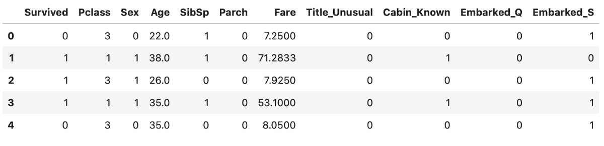
Image by author
This looks much better. There are still some things we could do, but let’s call it a day and proceed with the modeling.
Model selection and training
To start, let’s import the classification module from the PyCaret library and perform a basic setup:
from pycaret.classification import *
clf = setup(data, target='Survived', session_id=42)
I’ve set the random seed to 42, so you can reproduce the results.
After a couple of seconds, you’ll see a success message on the screen alongside a table that shows a bunch of information on your data. Read through it if you wish. Next, we will compare the performance of various machine learning models and see which one does the best overall:
compare_models()
Yes, it is as simple as a function call. Execution will take anywhere from a couple of seconds to a minute because several algorithms are trained with cross-validation. Once done, you should see this table:
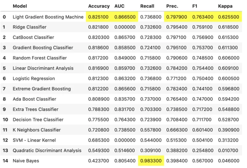
Image by author
It seems like Light Gradient Boosting approach did the best overall, so we can use it to create our model:
model = create_model('lightgbm')
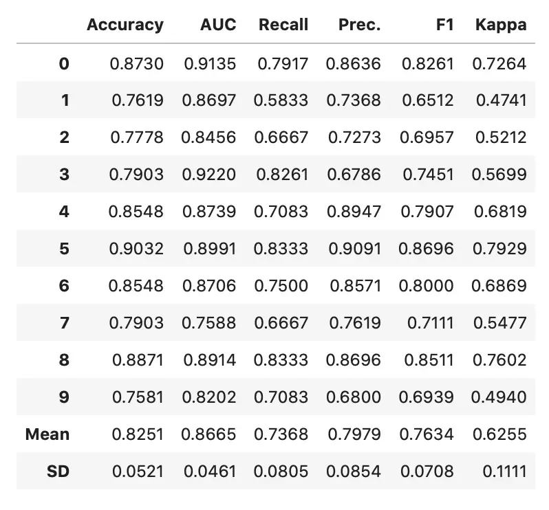
Image by author
You are free to perform additional hyperparameter tuning through the tune_model() function, but it didn’t improve the performance in my case.
We’ll make a couple of visualizations and interpretations in the next section.
Model visualization and interpretation
To start, let’s see what the plot_model() function has to offer:
plot_model(model)
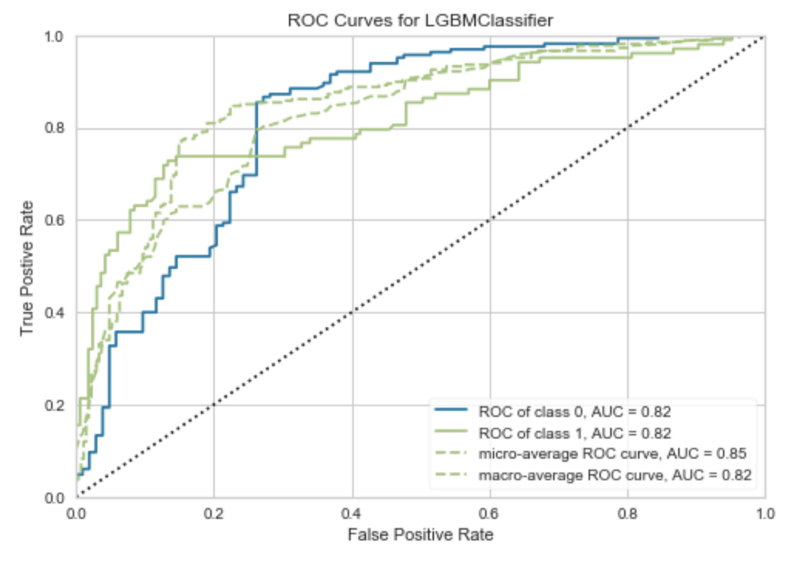
Image by author
Area under ROC (Receiver Operating Characteristics) curve tells us how good the model is at distinguishing between classes — predicting survived as survived, and died as died.
If this still isn’t quite interpretable as you would wish, here’s how to plot the confusion matrix:
plot_model(model, 'confusion_matrix')
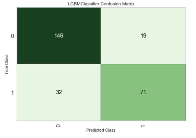
Image by author
The model is actually pretty decent if we take into account how easy it was to build it. Next, let’s use SHAP values to explain our model.
SHAP, or SHapley Additive exPlanations, is a way to explain the outputs of a machine learning model. We can use it to see which features are most important by plotting the SHAP values of every feature for every sample.
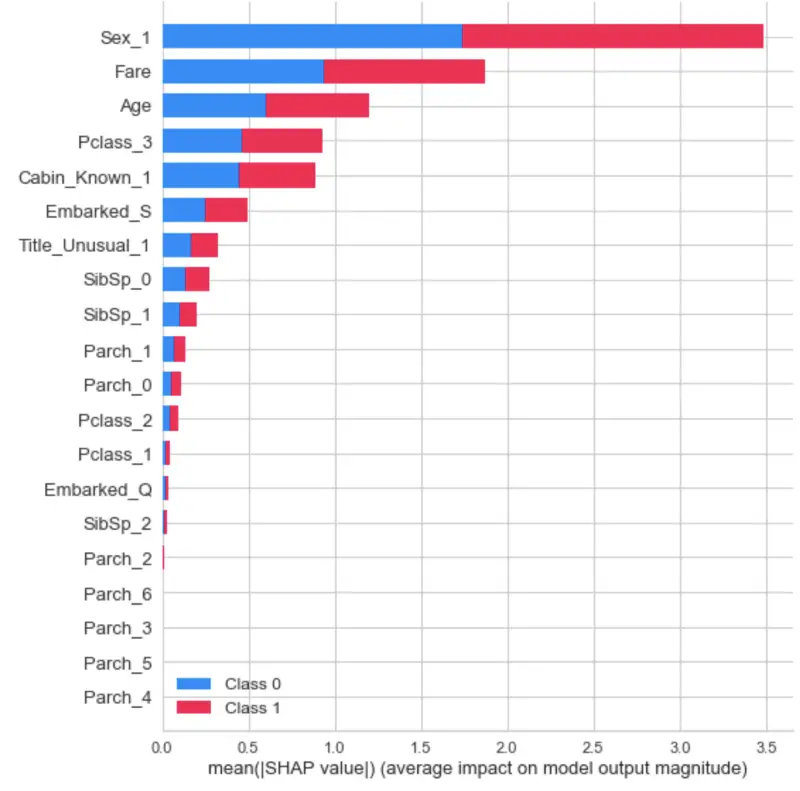
Image by author
Great! Let’s now make a final evaluation on the test set and save the model to a file.
Predictions and saving the model
Once we’re satisfied with how the model behaves, we can evaluate it on the test set (previously unseen data):
predictions = predict_model(model)
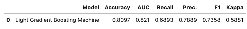
Image by author
When we called the setup() function, at the beginning of the article, PyCaret performed the train/test split in the 70:30 ratio. This ratio can be changed, of course, but I’m satisfied with the default.
The results are a bit worse on the test set, but that’s expected. Before saving the model to a file, we need to finalize it:
finalize_model(model)
Now the model can be saved:
save_model(model, 'titanic_lgbm')
The model is now saved in the same folder where the notebook is. To load it later, you would use the load_model() function with a file path as an argument.
Conclusion
I hope you’ve followed along, spent some more time on data preparation, and got a better model as a result. PyCaret sure does a lot of the things for us, so we can spend our time doing more important things.
There’s a lot more to explore, and that’s coming soon. Thanks for reading.