Machine Learning can be easy and intuitive — here’s a complete from-scratch guide to Simple Linear Regression
Linear regression is the simplest algorithm you’ll encounter while studying machine learning. If we’re talking about simple linear regression, you only need to find values for two parameters — slope and the intercept — but more on that in a bit.
Today you’ll get your hands dirty implementing simple linear regression algorithm from scratch. This is the first of many upcoming from scratch articles, so stay tuned to the blog if you want to learn more.
Today’s article is structured as follows:
- Introduction to Simple Linear Regression
- Math Behind Simple Linear Regression
- From-Scratch Implementation
- Comparison with Scikit-Learn
- Conclusion
You can download the corresponding notebook here.
Introduction to Simple Linear Regression
As the name suggests, simple linear regression is simple. It’s an algorithm used by many in introductory machine learning, but it doesn’t require any “learning”. It’s as simple as plugging few values into a formula — more on that in the following section.
In general, linear regression is used to predict continuous variables — something such as stock price, weight, and similar.
Linear regression is a linear algorithm, meaning the linear relationship between input variables (what goes in) and the output variable (the prediction) is assumed. It’s not the end of the world if the relationships in your dataset aren’t linear, as there’s plenty of conversion methods.
Several types of linear regression models exist:
- Simple linear regression— has a single input variable and a single output variable. For example, using height to predict the weight.
- Multiple linear regression— has multiple input variables and a single output variable. For example, using height, body fat, and BMI to predict weight.
Today we’ll deal with simple linear regression. The article on multiple linear regression is coming out next week, so stay tuned to the blog if you want to learn more.
Linear regression is rarely used as a go-to algorithm for solving complex machine learning problems. Instead, it’s used as a baseline model — a point which more sophisticated algorithms have to outperform.
The algorithm is also rather strict on the requirements. Let’s list and explain a few:
- Linear Assumption— model assumes the relationship between variables is linear
- No Noise— model assumes that the input and output variables are not noisy — so remove outliers if possible
- No Collinearity— model will overfit when you have highly correlated input variables
- Normal Distribution— the model will make more reliable predictions if your input and output variables are normally distributed. If that’s not the case, try using some transforms on your variables to make them more normal-looking
- Rescaled Inputs— use scalers or normalizer to make more reliable predictions
You now know enough theory behind this simple algorithm. Let’s look at the math next before the implementation.
Math Behind Simple Linear Regression
In essence, simple linear regression boils down to solving a couple of equations. You only need to solve the line equation, displayed in the following figure:

Image 1 — Line equation formula (image by author)
As you can see, we need to calculate the beta coefficients somehow. X represents input data, so that’s something you already have at your disposal.
The Beta 1 coefficient has to be calculated first. It represents the slope of the line and can be obtained with the following formula:

Image 2 — Beta 1 coefficient in the line equation (image by author)
The Xi represents the current value of the input feature, and X with a bar on top represents the mean of the entire variable. The same goes with Y, but we’re looking at the target variable instead.
Next, we have the Beta 0 coefficient. You can calculate it with the following formula:

Image 3 — Beta 0 coefficient in the line equation (image by author)
And that’s all there is to simple linear regression! Once the coefficient values are calculated, you can plug in the number for X and get the prediction. As simple as that.
Let’s take a look at the Python implementation next.
From-Scratch Implementation
Let’s start with the library imports. You’ll only need Numpy and Matplotlib for now. The rcParams modifications are optional, only to make the visuals look a bit better:
import numpy as np
import matplotlib.pyplot as plt
from matplotlib import rcParams
rcParams['figure.figsize'] = (14, 7)
rcParams['axes.spines.top'] = False
rcParams['axes.spines.right'] = False
Now onto the algorithm implementation. Let’s declare a class called SimpleLinearRegression with the following methods:
__init__()– the constructor, contains the values for Beta 0 and Beta 1 coefficients. These are initially set toNonefit(X, y)– calculates the Beta 0 and Beta 1 coefficients from the inputXandyparameters. After the calculation is done, the results are stored in the constructorpredict(X)– makes the prediction using the line equation. It throws an error if thefit()method wasn’t called beforehand.
If you understand the math behind this simple algorithm, implementation in Python is easy. Here’s the entire code snippet for the class:
class SimpleLinearRegression:
    '''
    A class which implements simple linear regression model.
    '''
    def __init__(self):
        self.b0 = None
        self.b1 = None

    def fit(self, X, y):
        '''
        Used to calculate slope and intercept coefficients.

        :param X: array, single feature
        :param y: array, true values
        :return: None
        '''
        numerator = np.sum((X - np.mean(X)) * (y - np.mean(y)))
        denominator = np.sum((X - np.mean(X)) ** 2)
        self.b1 = numerator / denominator
        self.b0 = np.mean(y) - self.b1 * np.mean(X)

    def predict(self, X):
        '''
        Makes predictions using the simple line equation.

        :param X: array, single feature
        :return: None
        '''
        if not self.b0 or not self.b1:
            raise Exception('Please call `SimpleLinearRegression.fit(X, y)` before making predictions.')
        return self.b0 + self.b1 * X
Next, let’s create some dummy data. We’ll make a range of 300 data points as the input variable, and 300 normally distributed values as the target variable. The target variable is centered around the input variable, with a standard deviation of 20.
You can use the following code snippet to create and visualize the dataset:
X = np.arange(start=1, stop=301)
y = np.random.normal(loc=X, scale=20)

plt.scatter(X, y, s=200, c='#087E8B', alpha=0.65)
plt.title('Source dataset', size=20)
plt.xlabel('X', size=14)
plt.ylabel('Y', size=14)
plt.savefig('images/001_SimpleLinearRegression_source_dataset.png', dpi=300, bbox_inches='tight')
plt.show()
The visualization of the dataset is shown in the following figure:
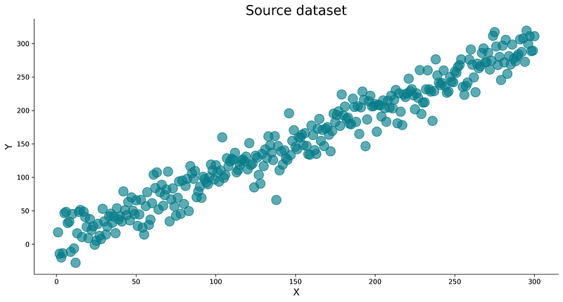
Image 4 — Source dataset (image by author)
Next, let’s split the dataset into training and testing subsets. You can use the train_test_split() function from Scikit-learn to do so:
from sklearn.model_selection import train_test_split

X_train, X_test, y_train, y_test = train_test_split(X, y, test_size=0.2, random_state=42)
Finally, let’s make an instance of the SimpleLinearRegression class, fit the training data, and make predictions on the test set. The following code snippet does just that, and also prints the values of Beta 0 and Beta 1 coefficients:
model = SimpleLinearRegression()
model.fit(X_train, y_train)
preds = model.predict(X_test)

model.b0, model.b1
The coefficient values are displayed below:

Image 5 — Beta 0 and Beta 1 coefficient values (image by author)
And that’s your line equation formula. Next, we need a way to evaluate the model. Before doing that, let’s quickly see how the preds and y_test variables look like.
Here’s what inside the preds variable:
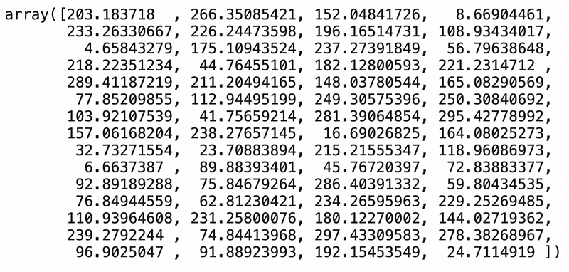
Image 6 — Predictions of a simple linear regression model (image by author)
And here’s how the actual test data looks like:
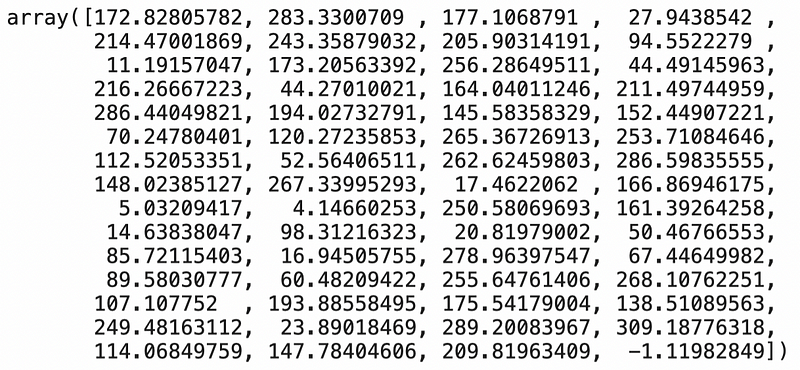
Image 7 — Actual values in the test set (image by author)
Not identical, sure, but quite similar overall. For a more quantitative evaluation metric, we’ll use RMSE (Root Mean Squared Error). Here’s how to calculate its value with Python:
from sklearn.metrics import mean_squared_error

rmse = lambda y, y_pred: np.sqrt(mean_squared_error(y, y_pred))
rmse(y_test, preds)
The average error is displayed below:

Image 8 — Root Mean Squared Error on the test set (image by author)
As you can see, our model is around 20 units wrong on average. That’s due to introduced variance when declaring the dataset, so there’s nothing we can do to improve the model further.
If you want to visualize the best fit line, you’d have to retrain the model on the entire dataset and plot the predictions. You can do so with the following code snippet:
model_all = SimpleLinearRegression()
model_all.fit(X, y)
preds_all = model_all.predict(X)

plt.scatter(X, y, s=200, c='#087E8B', alpha=0.65, label='Source data')
plt.plot(X, preds_all, color='#000000', lw=3, label=f'Best fit line > B0 = {model_all.b0:.2f}, B1 = {model_all.b1:.2f}')
plt.title('Best fit line', size=20)
plt.xlabel('X', size=14)
plt.ylabel('Y', size=14)
plt.legend()
plt.show()
Here’s how it looks like:
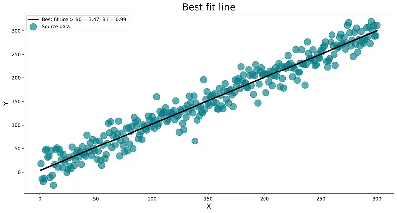
Image 9 — Best fit line on the entire dataset (image by author)
And that’s all there is to a simple linear regression model. Let’s compare it to a LinearRegression class from Scikit-Learn and see if there are any severe differences.
Comparison with Scikit-Learn
We want to know if our model is any good, so let’s compare it with something we know works well — a LinearRegression class from Scikit-Learn.
You can use the following snippet to import the class, train the model, make predictions, and print the values for Beta 0 and Beta 1 coefficients:
from sklearn.linear_model import LinearRegression

sk_model = LinearRegression()
sk_model.fit(np.array(X_train).reshape(-1, 1), y_train)
sk_preds = sk_model.predict(np.array(X_test).reshape(-1, 1))

sk_model.intercept_, sk_model.coef_
The coefficient values are displayed below:

Image 10 — Beta 0 and Beta 1 coefficients from the Scikit-Learn model (image by author)
As you can see, the coefficients are nearly identical! Next, let’s check the RMSE value:
rmse(y_test, sk_preds)

Image 11 — Root Mean Squared Error of a Scikit-Learn model (image by author)
Once again, nearly identical! Model quality — check.
Let’s wrap things up in the next section.
Conclusion
Today you’ve learned how to implement simple linear regression algorithm in Python entirely from scratch.
Does that mean you should ditch the de facto standard machine learning libraries? No, not at all. Let me elaborate.
Just because you can write something from scratch doesn’t mean you should. Still, knowing every detail of how algorithms work is a valuable skill and can help you stand out from every other fit and predict data scientist.
Thanks for reading, and please stay tuned to the blog if you’re interested in more machine learning from scratch articles.
Stay connected
- Sign up for my newsletter
- Subscribe on YouTube
- Connect on LinkedIn

