
Machine Learning can be easy and intuitive — here’s a complete from-scratch guide to Multiple Linear Regression
Linear regression is the simplest algorithm you’ll encounter while studying machine learning. Multiple linear regression is similar to the simple linear regression covered last week — the only difference being multiple slope parameters. How many? Well, that depends on how many input features there are — but more on that in a bit.
Today you’ll get your hands dirty implementing multiple linear regression algorithm from scratch. This is the second of many upcoming from scratch articles, so stay tuned to the blog if you want to learn more.
Today’s article is structured as follows:
- Introduction to Multiple Linear Regression
- Math Behind Multiple Linear Regression
- From-Scratch Implementation
- Comparison with Scikit-Learn
- Conclusion
You can download the corresponding notebook here.
Introduction to Multiple Linear Regression
Multiple linear regression shares the same idea as its simple version — to find the best fitting line (hyperplane) given the input data. What makes it different is the ability to handle multiple input features instead of just one.
The algorithm is rather strict on the requirements. Let’s list and explain a few:
- Linear Assumption— model assumes the relationship between variables is linear
- No Noise— model assumes that the input and output variables are not noisy — so remove outliers if possible
- No Collinearity— model will overfit when you have highly correlated input variables
- Normal Distribution— the model will make more reliable predictions if your input and output variables are normally distributed. If that’s not the case, try using some transforms on your variables to make them more normal-looking
- Rescaled Inputs— use scalers or normalizer to make more reliable predictions
Training multiple linear regression model means calculating the best coefficients for the line equation formula. The best coefficients can be calculated through an iterative optimization process, known as gradient descent.
This algorithm calculates the derivates with respect to each coefficient and updates them on each iteration. How much of an update there will be depends on one parameter — learning rate. A high learning rate can lead to “missing” the best parameter values, and a low learning rate can lead to slow optimization.
More on that in the next section, where we’ll discuss the math behind the algorithm.
Math Behind Multiple Linear Regression
The math behind multiple linear regression is a bit more complicated than it was for the simple one, as you can’t simply plug the values into a formula. We’re dealing with an iterative process instead.
The equation we’re solving remains more or less the same:
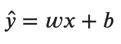
Image 1 — Multiple linear regression formula (image by author)
We don’t have a single beta coefficient for the slope, but instead, we have an entire matrix of them — denoted as w for weights. There’s still a single intercept value — denoted as b for bias.
We’ll have to declare a cost function to continue. This is a function that measures error and represents something we want to minimize. Mean squared error (MSE) is the most common cost function for linear regression:
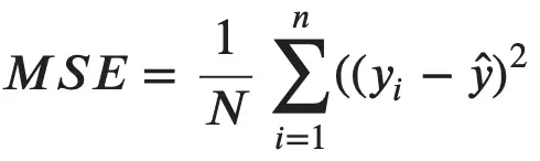
Image 2 — Mean squared error formula (image by author)
Put simply, it represents the average square difference between actual (yi) and predicted (_y ha_t) values. The y hat can be expanded into the following:
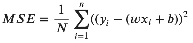
Image 3 — Mean squared error formula (v2) (image by author)
As mentioned before, we’ll use the gradient descent algorithm to find optimal weights and bias. It relies on partial derivative calculation for each parameter. You can find derived MSE formulas with respect to each parameter below:
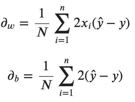
Image 4 — MSE partial derivatives (image by author)
Finally, the update process can be summarized into two formulas — one for each parameter. Put simply, old weight (or bias) values are subtracted from the product of learning rate and the derivative calculation:
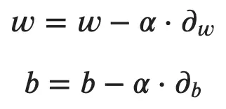
Image 5 — Update rules for multiple linear regression (image by author)
The alpha parameter represents the learning rate.
The entire process is repeated for the desired number of iterations. Let’s see how this works in practice, by implementing a from-scratch solution with Python.
From-Scratch Implementation
Let’s start with the library imports. You’ll only need Numpy and Matplotlib for now. The rcParams modifications are optional, only to make the visuals look a bit better:
import numpy as np
import matplotlib.pyplot as plt
from matplotlib import rcParams
rcParams['figure.figsize'] = (14, 7)
rcParams['axes.spines.top'] = False
rcParams['axes.spines.right'] = False
Onto the algorithm now. Let’s declare a class called LinearRegression with the following methods:
__init__()– the constructor, contains the values for learning rate and the number of iterations, alongside the weights and bias (initially set to None). We’ll also create an empty list to track loss at each iteration._mean_squared_error(y, y_hat)– “private” method, used as our cost function.fit(X, y)– iteratively optimizes weights and bias through gradient descent. After the calculation is done, the results are stored in the constructor. We’re also keeping track of loss here.predict(X)– makes the prediction using the line equation.
If you understand the math behind this simple algorithm, implementation in Python is easy. Here’s the entire code snippet for the class:
class LinearRegression:
    '''
    A class which implements linear regression model with gradient descent.
    '''
    def __init__(self, learning_rate=0.01, n_iterations=10000):
        self.learning_rate = learning_rate
        self.n_iterations = n_iterations
        self.weights, self.bias = None, None
        self.loss = []

    @staticmethod
    def _mean_squared_error(y, y_hat):
        '''
        Private method, used to evaluate loss at each iteration.

        :param: y - array, true values
        :param: y_hat - array, predicted values
        :return: float
        '''
        error = 0
        for i in range(len(y)):
            error += (y[i] - y_hat[i]) ** 2
        return error / len(y)

    def fit(self, X, y):
        '''
        Used to calculate the coefficient of the linear regression model.

        :param X: array, features
        :param y: array, true values
        :return: None
        '''
        # 1. Initialize weights and bias to zeros
        self.weights = np.zeros(X.shape[1])
        self.bias = 0

        # 2. Perform gradient descent
        for i in range(self.n_iterations):
            # Line equation
            y_hat = np.dot(X, self.weights) + self.bias
            loss = self._mean_squared_error(y, y_hat)
            self.loss.append(loss)

            # Calculate derivatives
            partial_w = (1 / X.shape[0]) * (2 * np.dot(X.T, (y_hat - y)))
            partial_d = (1 / X.shape[0]) * (2 * np.sum(y_hat - y))

            # Update the coefficients
            self.weights -= self.learning_rate * partial_w
            self.bias -= self.learning_rate * partial_d


    def predict(self, X):
        '''
        Makes predictions using the line equation.

        :param X: array, features
        :return: array, predictions
        '''
        return np.dot(X, self.weights) + self.bias
Let’s test the algorithm next. We’ll use the Diabetes dataset from Scikit-Learn. The following code snippet loads the dataset and splits it into features and target arrays:
from sklearn.datasets import load_diabetes

data = load_diabetes()
X = data.data
y = data.target
The next step is to split the dataset into training and testing subsets and to train the model. You can do so with the following code snippet:
from sklearn.model_selection import train_test_split

X_train, X_test, y_train, y_test = train_test_split(X, y, test_size=0.2, random_state=42)

model = LinearRegression()
model.fit(X_train, y_train)
preds = model.predict(X_test)
Here’s how the “optimal” weight matrix looks like:
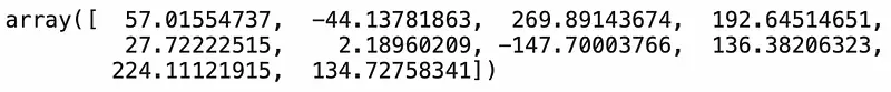
Image 6 — Optimized weight matrix (image by author)
And here’s the optimal value for our bias term:
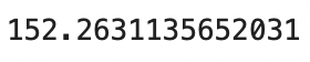
Image 7 — Optimized bias term (image by author)
And that’s all there is to it! You’ve successfully trained the model for 10000 iterations and landed on a hopefully good set of parameters. Let’s see how good they are by plotting the loss:
xs = np.arange(len(model.loss))
ys = model.loss

plt.plot(xs, ys, lw=3, c='#087E8B')
plt.title('Loss per iteration (MSE)', size=20)
plt.xlabel('Iteration', size=14)
plt.ylabel('Loss', size=14)
plt.show()
Ideally, we should see a line that starts at a high loss value and quickly drops to somewhere near zero:
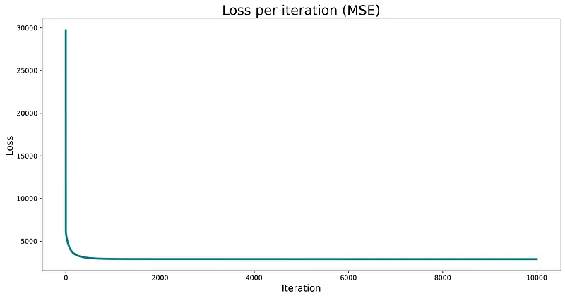
Image 8 — Loss per iteration (image by author)
It looks promising, but how can we know if the loss is low enough to produce a good quality model? Well, we can’t, at least not directly. The best thing we can do loss-wise is to train a couple of models with different learning rates and compare loss curves. The following code snippet does just that:
losses = {}
for lr in [0.5, 0.1, 0.01, 0.001]:
    model = LinearRegression(learning_rate=lr)
    model.fit(X_train, y_train)
    losses[f'LR={str(lr)}'] = model.loss


xs = np.arange(len(model.loss))

plt.plot(xs, losses['LR=0.5'], lw=3, label=f"LR = 0.5, Final = {losses['LR=0.5'][-1]:.2f}")
plt.plot(xs, losses['LR=0.1'], lw=3, label=f"LR = 0.1, Final = {losses['LR=0.1'][-1]:.2f}")
plt.plot(xs, losses['LR=0.01'], lw=3, label=f"LR = 0.01, Final = {losses['LR=0.01'][-1]:.2f}")
plt.plot(xs, losses['LR=0.001'], lw=3, label=f"LR = 0.001, Final = {losses['LR=0.001'][-1]:.2f}")
plt.title('Loss per iteration (MSE) for different learning rates', size=20)
plt.xlabel('Iteration', size=14)
plt.ylabel('Loss', size=14)
plt.legend()
plt.show()
The results are shown below:
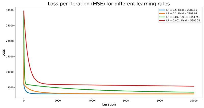
Image 9 — Loss comparison for different learning rates (image by author)
It seems like a learning rate of 0.5 works the best for our data. You can retrain the model to accommodate with the following code snippet:
model = LinearRegression(learning_rate=0.5)
model.fit(X_train, y_train)
preds = model.predict(X_test)

model._mean_squared_error(y_test, preds)
Here’s the corresponding MSE value on the test set:
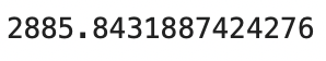
Image 10 — Mean squared error on the test set (image by author)
And that’s how easy it is to build, train, evaluate, and tweak a multiple linear regression model from scratch! Let’s compare it to a LinearRegression class from Scikit-Learn and see if there are any severe differences.
Comparison with Scikit-Learn
We want to know if our model is any good, so let’s compare it with something we know works well — a LinearRegression class from Scikit-Learn.
You can use the following snippet to import the model class, train the model, make predictions, and print the value of the mean squared error on the test set:
from sklearn.linear_model import LinearRegression
from sklearn.metrics import mean_squared_error

lr_model = LinearRegression()
lr_model.fit(X_train, y_train)
lr_preds = lr_model.predict(X_test)

mean_squared_error(y_test, lr_preds)
Here is the corresponding MSE value:
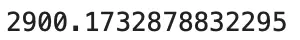
Image 11 — Mean squared error with Scikit-Learn model (image by author)
As you can see, our tweaked model outperformed the default one from Scikit-Learn, but the difference isn’t significant. Model quality — check.
Let’s wrap things up in the next section.
Conclusion
Today you’ve learned how to implement multiple linear regression algorithm in Python entirely from scratch. Does that mean you should ditch the de facto standard machine learning libraries? No, not at all. Let me elaborate.
Just because you can write something from scratch doesn’t mean you should. Still, knowing every detail of how algorithms work is a valuable skill and can help you stand out from every other fit and predict data scientist.
Thanks for reading, and please stay tuned to the blog if you’re interested in more machine learning from scratch articles.
Stay connected
- Sign up for my newsletter
- Subscribe on YouTube
- Connect on LinkedIn