
Machine Learning can be easy and intuitive — here’s a complete from-scratch guide to Logistic Regression
Logistic regression is the simplest classification algorithm you’ll ever encounter. It’s similar to the linear regression explored last week, but with a twist. More on that in a bit.
Today you’ll get your hands dirty by implementing and tweaking the logistic regression algorithm from scratch. This is the third of many upcoming from-scratch articles, so stay tuned to the blog if you want to learn more. The links to the previous articles are located at the end of this piece.
The article is structured as follows:
- Introduction to Logistic Regression
- Math Behind Logistic Regression
- Introduction to Binary Cross Entropy Loss
- From-Scratch Implementation
- Threshold Optimization
- Comparison with Scikit-Learn
- Conclusion
You can download the corresponding notebook here.
Introduction to Logistic Regression
Logistic regression is a fundamental machine learning algorithm for binary classification problems. Nowadays, it’s commonly used only for constructing a baseline model. Still, it’s an excellent first algorithm to build because it’s highly interpretable.
In a way, logistic regression is similar to linear regression. We’re still dealing with a line equation for making predictions. This time, the results are passed through a Sigmoid activation function to convert real values to probabilities.
The probability tells you the chance of the instance belonging to a positive class (e.g., this customer has a 0.85 churn probability). These probabilities are then turned to actual classes based on a threshold value. If the probability is greater than the threshold, we assign the positive class and vice-versa.
The threshold value can (and should) be altered depending on the problem and the type of metric you’re optimizing for.
Let’s talk about assumptions of a logistic regression model[1]:
- The observations (data points) are independent
- There is little to no multicollinearity among independent variables (check for correlation and remove for redundancy)
- Large sample size — a minimum of 10 cases with the least frequent outcome for each independent variable. For example, if you have five independent variables and the expected probability of the least frequency outcome is 0.1, then you need a minimum sample size of 500 (10 * 5 / 0.1)
Training a logistic regression model means calculating the best coefficients for weights and bias. These can be calculated through an iterative optimization process known as gradient descent. More on that in the next section.
Math Behind Logistic Regression
The math behind logistic regression is quite simple. We’re still dealing with a line equation:
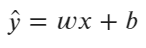
Image 1 — Line equation formula (image by author)
But this time, the output of the line equation is passed through a Sigmoid (Logistic) function, shown in the following formula:
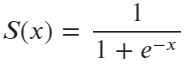
Image 2 — Sigmoid function formula (image by author)
The role of a sigmoid function is to take any real value and map it to a probability — value between zero and one. It’s an S-shaped function, and you can use the following code to visualize it:
import numpy as np
import matplotlib.pyplot as plt
from matplotlib import rcParams
rcParams['figure.figsize'] = (14, 7)
rcParams['axes.spines.top'] = False
rcParams['axes.spines.right'] = False


def sigmoid(x):
    return 1 / (1 + np.exp(-x))

xs = np.arange(-10, 10, 0.1)
ys = [sigmoid(x) for x in xs]

plt.plot(xs, ys, c='#087E8B', lw=3)
plt.title('Sigmoid function', size=20)
plt.xlabel('X', size=14)
plt.ylabel('Y (probability)', size=14)
plt.show()
Here’s the visualization:
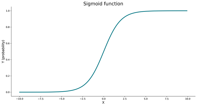
Image 3 — Sigmoid function (image by author)
The value the sigmoid function returns is interpreted as a probability of the positive class. If the probability is larger than some threshold (commonly 0.5), we assign the positive class. If the probability is lower than the threshold, we assign the negative class.
As with linear regression, there are two parameters we need to optimize for — weights and bias. We’ll need to declare the cost function to perform the optimization. Unfortunately, the familiar mean squared error function can’t be used. Well, it can be used in theory, but it isn’t a good idea.
Instead, we’ll use a Binary Cross Entropy function, shown in the following formula:
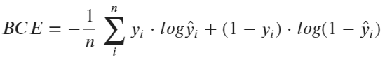
Image 4 — Binary cross-entropy loss formula (image by author)
Don’t worry if it looks like a foreign language, we’ll explain it in the next section.
Next, you’ll need to use this cost function in the optimization process to update weights and bias iteratively. To do so, you’ll have to calculate partial derivatives of the binary cross entropy function concerning weights and bias parameters:
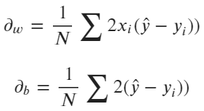
Image 5 — Binary cross-entropy derivatives (image by author)
The scalar can be omitted, as it doesn’t make any difference. Next, you’ll have to update the existing weights and bias according to the update rules — shown in the following formulas:
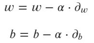
Image 6 — Gradient descent update rules (image by author)
The alpha parameter represents the learning rate. The entire process is repeated for the desired number of iterations.
And that’s all with regards to the math! Let’s go over the binary cross entropy loss function next.
Introduction to Binary Cross Entropy Loss
Binary cross entropy is a common cost (or loss) function for evaluating binary classification models. It’s commonly referred to as log loss, so keep in mind these are synonyms.
This cost function “punishes” wrong predictions much more than it “rewards” good ones. Let’s see it in action.
Example 1 — Calculating BCE for a correct prediction
Let’s say your model predicts the positive class with a 90% probability (0.9). This means the model is only 10% confident the negative class should be predicted.
Question: What’s the BCE value?
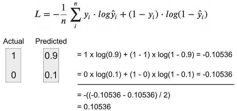
Image 7 — Binary cross-entropy calculation — example 1 (image by author)
As you can see, the BCE value is rather small, only 0.1. This is because the model was pretty confident in the prediction. Let’s see what happens if that’s not the case.
Example 2 — Calculating BCE for an incorrect prediction
Let’s say your model predicts the positive class with a 10% probability (0.1). This means the model is 90% confident the negative class should be predicted.
Question: What is the BCE value?
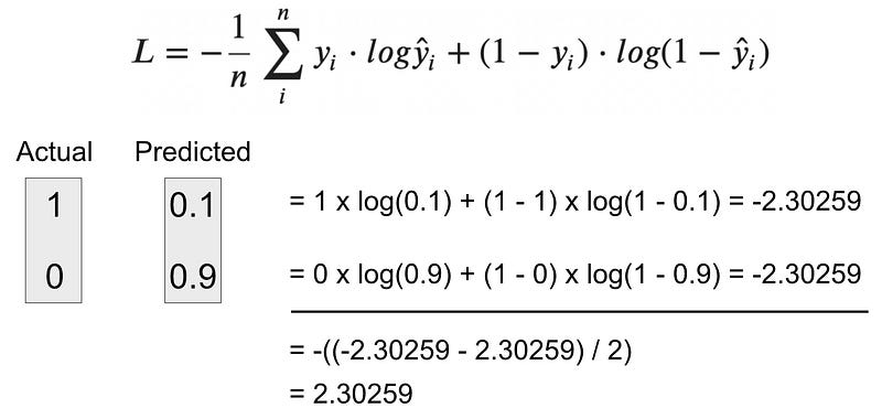
Image 8 — Binary cross-entropy calculation — example 2 (image by author)
As you can see, the loss is quite big in this case — a perfect demonstration of how BCE punishes the wrong prediction much more than it rewards the good ones.
Python implementation
I’m not a big fan of doing math by hand. If the same applies to you, you’ll like this part. The following function implements BCE from scratch in Python:
def binary_cross_entropy(y, y_hat):
    def safe_log(x): return 0 if x == 0 else np.log(x)

    total = 0
    for curr_y, curr_y_hat in zip(y, y_hat):
        total += (curr_y * safe_log(curr_y_hat) + (1 - curr_y) * safe_log(1 - curr_y_hat))
    return - total / len(y)


print(binary_cross_entropy(y=[1, 0], y_hat=[0.9, 0.1]))
print(binary_cross_entropy(y=[1, 0], y_hat=[0.1, 0.9]))
We need the safe_log() function because log(0) equals infinity. Anyhow, you’ll see that our by-hand calculations were correct if you run this code.
You now know everything needed to implement a logistic regression algorithm from scratch. Let’s do that next.
From-Scratch Implementation
Let the fun part begin! We’ll now declare a class called LogisticRegression with the following methods:
__init__(learning_rate, n_iterations)– the constructor, contains the values for learning rate and the number of iterations, alongside the weights and bias (initially set to None)_sigmoid(x)– logistic activation function, you know the formula_binary_cross_entropy(y, y_hat)– our cost function – we implemented it earlier alreadyfit(X, y)– iteratively optimizes weights and bias through gradient descent. After the calculation is done, the results are stored in the constructorpredict_proba(X)– calculates the prediction probabilities using the line equations passed through a sigmoid activation functionpredict(X, threshold)– calculates predicted classes (binary) based on the threshold parameter
If you understand the math behind logistic regression, implementation in Python should be an issue. It all boils down to around 70 lines of documented code:
class LogisticRegression:
    '''
    A class which implements logistic regression model with gradient descent.
    '''
    def __init__(self, learning_rate=0.1, n_iterations=1000):
        self.learning_rate = learning_rate
        self.n_iterations = n_iterations
        self.weights, self.bias = None, None

    @staticmethod
    def _sigmoid(x):
        '''
        Private method, used to pass results of the line equation through the sigmoid function.

        :param x: float, prediction made by the line equation
        :return: float
        '''
        return 1 / (1 + np.exp(-x))

    @staticmethod
    def _binary_cross_entropy(y, y_hat):
        '''
        Private method, used to calculate binary cross entropy value between actual classes
        and predicted probabilities.

        :param y: array, true class labels
        :param y_hat: array, predicted probabilities
        :return: float
        '''
        def safe_log(x):
            return 0 if x == 0 else np.log(x)
        total = 0
        for curr_y, curr_y_hat in zip(y, y_hat):
            total += (curr_y * safe_log(curr_y_hat) + (1 - curr_y) * safe_log(1 - curr_y_hat))
        return - total / len(y)

    def fit(self, X, y):
        '''
        Used to calculate the coefficient of the logistic regression model.

        :param X: array, features
        :param y: array, true values
        :return: None
        '''
        # 1. Initialize coefficients
        self.weights = np.zeros(X.shape[1])
        self.bias = 0

        # 2. Perform gradient descent
        for i in range(self.n_iterations):
            linear_pred = np.dot(X, self.weights) + self.bias
            probability = self._sigmoid(linear_pred)

            # Calculate derivatives
            partial_w = (1 / X.shape[0]) * (2 * np.dot(X.T, (probability - y)))
            partial_d = (1 / X.shape[0]) * (2 * np.sum(probability - y))

            # Update the coefficients
            self.weights -= self.learning_rate * partial_w
            self.bias -= self.learning_rate * partial_d

    def predict_proba(self, X):
        '''
        Calculates prediction probabilities for a given threshold using the line equation
        passed through the sigmoid function.

        :param X: array, features
        :return: array, prediction probabilities
        '''
        linear_pred = np.dot(X, self.weights) + self.bias
        return self._sigmoid(linear_pred)

    def predict(self, X, threshold=0.5):
        '''
        Makes predictions using the line equation passed through the sigmoid function.

        :param X: array, features
        :param threshold: float, classification threshold
        :return: array, predictions
        '''
        probabilities = self.predict_proba(X)
        return [1 if i > threshold else 0 for i in probabilities]
Let’s test the algorithm next. We’ll use the Breast cancer dataset from Scikit-Learn. The following code snippet loads it, makes a train/test split in 80:20 ratio, instantiates the model, fits the data, and makes predictions:
from sklearn.datasets import load_breast_cancer
from sklearn.model_selection import train_test_split

data = load_breast_cancer()
X = data.data
y = data.target

X_train, X_test, y_train, y_test = train_test_split(X, y, test_size=0.2, random_state=42)

model = LogisticRegression()
model.fit(X_train, y_train)
preds = model.predict(X_test)
In case you want to know, here are the values for the optimal weights (accessed through model.weights):
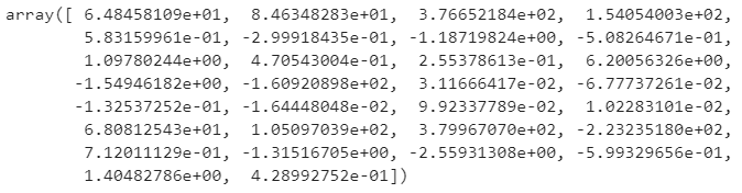
Image 9 — Optimized weights (image by author)
And here’s the optimal bias (accessed through model.bias):
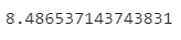
Image 10 — Optimized bias (image by author)
This concludes the training portion. Let’s evaluate the model next.
Model evaluation
We’ll keep things simple here and print only the accuracy score and the confusion matrix. You can use the following code snippet to do so:
from sklearn.metrics import accuracy_score, confusion_matrix

print(accuracy_score(y_test, preds))
print(confusion_matrix(y_test, preds))
Here’s the accuracy value:
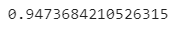
Image 11 — Initial accuracy (image by author)
And here’s the confusion matrix:

Image 12 — Initial confusion matrix (image by author)
As you can see, the model works just fine with around 95% accuracy. There are six false negatives, meaning that in six cases model predicted “No” when the actual condition was “Yes”. Still, more than decent results.
Let’s explore how you can make the results even better by tweaking the classification threshold.
Threshold Optimization
There’s no guarantee that 0.5 is the best classification threshold for every classification problem. Luckily, we can change the threshold by altering the threshold parameter of the predict() method.
The following code snippet optimizes the threshold for accuracy, but you’re free to choose any other metric:
import pandas as pd

evals = []
for thresh in np.arange(0, 1.01, 0.01):
    preds = model.predict(X_test, threshold=thresh)
    acc = accuracy_score(y_test, preds)
    evals.append({'Threshold': thresh, 'Accuracy': acc})

evals_df = pd.DataFrame(evals)
best_thresh = evals_df.sort_values(by='Accuracy', ascending=False).iloc[0]

plt.plot(evals_df['Threshold'], evals_df['Accuracy'], lw=3, c='#087E8B')
plt.scatter(best_thresh['Threshold'], best_thresh['Accuracy'], label=f"Best threshold = {best_thresh['Threshold']}, Accuracy = {(best_thresh['Accuracy'] * 100):.2f}%", s=250, c='#087E8B')
plt.title('Threshold Optimization', size=20)
plt.xlabel('Threshold', size=14)
plt.ylabel('Accuracy', size=14)
plt.legend()
plt.show()
Here’s how the threshold chart looks like:
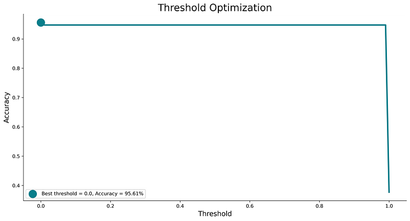
Image 13 — Threshold optimization curve (image by author)
The best threshold and the corresponding obtained accuracy are shown in the plot legend. As you can see, the threshold value is more or less irrelevant for this dataset, but that likely won’t be the case for other datasets.
You can now quickly retrain the model with the optimal threshold value in mind:
model = LogisticRegression()
model.fit(X_train, y_train)
preds = model.predict(X_test, threshold=0)

print(accuracy_score(y_test, preds))
print(confusion_matrix(y_test, preds))
Here’s the new, improved accuracy score:
Image 14 — Optimized accuracy (image by author)
And here’s the confusion matrix:

Image 15 — Optimized confusion matrix (image by author)
Now you know how to train a custom classifier model and how to optimize the classification threshold. Let’s compare it to a Scikit-Learn model next.
Comparison with Scikit-Learn
We want to know if our model is any good, so let’s compare it with something we know works well — a LogisticRegression class from Scikit-Learn.
You can use the following snippet to import the model class, train the model, make predictions, and print accuracy and confusion matrix:
from sklearn.linear_model import LogisticRegression

lr_model = LogisticRegression()
lr_model.fit(X_train, y_train)
lr_preds = lr_model.predict(X_test)

print(accuracy_score(y_test, lr_preds))
print(confusion_matrix(y_test, lr_preds))
Here’s the obtained accuracy score:
Image 16 — Accuracy from a Scikit-Learn model (image by author)
And here’s the confusion matrix:

Image 17 — Confusion matrix from a Scikit-Learn model (image by author)
As you can see, the model from Scikit-Learn performs roughly the same, at least accuracy-wise. There are some tradeoffs between false positives and false negatives, but in general, both models perform well.
Let’s wrap things up in the next section.
Conclusion
Today you’ve learned how to implement logistic regression in Python entirely from scratch. Does that mean you should ditch the de facto standard machine learning libraries? No, not at all. Let me elaborate.
Just because you can write something from scratch doesn’t mean you should. Still, knowing every detail of how algorithms work is a valuable skill and can help you stand out from every other fit and predict data scientist.
Thanks for reading, and please stay tuned to the blog if you’re interested in more machine learning from scratch articles.
Stay connected
- Sign up for my newsletter
- Subscribe on YouTube
- Connect on LinkedIn