
Machine Learning can be easy and intuitive — here’s a complete from-scratch guide to K Nearest Neighbors.
K Nearest Neighbors is one of the simplest, if not the simplest, machine learning algorithms. It is a classification algorithm that makes predictions based on a defined number of nearest instances.
Today you’ll get your hands dirty by implementing and tweaking the K nearest neighbors algorithm from scratch. This is the fourth of many upcoming from-scratch articles, so stay tuned to the blog if you want to learn more. The links to the previous articles are located at the end of this piece.
The article is structured as follows:
- Introduction to K Nearest Neighbors
- Math Behind K Nearest Neighbors
- From-Scratch Implementation
- K Optimization
- Comparison with Scikit-Learn
- Conclusion
You can download the corresponding notebook here.
Introduction to K Nearest Neighbors
As said earlier, K Nearest Neighbors is one of the simplest machine learning algorithms to implement. Its classification for a new instance is based on the target labels of K nearest instances, where K is a tunable hyperparameter.
Not only that, but K is the only mandatory hyperparameter. Changing its value can lead to an increase or decrease in model performance, depending on the data. You’ll learn how to find optimal K for any dataset today.
The strangest thing about the algorithm is that it doesn’t require any learning— but only a simple distance calculation. The choice of distance metric is up to you, but the most common ones are Euclidean and Cosine distances. We’ll work with Euclidean today.
When it comes to gotchas of using this algorithm, keep in mind it’s distance-based. Because of that, it might be a good idea to standardize your data before training.
And that’s pretty much all when it comes to the theory. Let’s talk briefly about the math behind before jumping into the code.
Math Behind K Nearest Neighbors
The distance calculation boils down to a single and simple formula. You aren’t obligated to use Euclidean distance, so keep that in mind.
The distance is calculated as a square root of squared differences between corresponding elements of two vectors. The vectors have to be of the same size, of course. Here’s the formula:
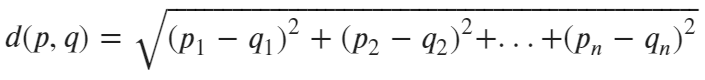
Image 1 — Euclidean distance formula v1 (image by author)
The formula can be written in a more compact way, as shown below:
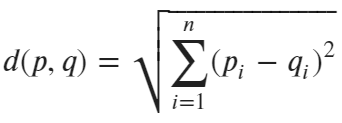
Image 2 — Euclidean distance formula v2 (image by author)
So keep in mind that these two mean the same.
And that’s the whole logic you need to implement in Python! Let’s do that next.
From-Scratch Implementation
Let’s start with the imports. We’ll need Numpy, Pandas, and Scipy for the logic and Matplotlib for visualization:
import numpy as np
import pandas as pd
import matplotlib.pyplot as plt
from scipy import stats
from matplotlib import rcParams
rcParams['axes.spines.top'] = False
rcParams['axes.spines.right'] = False
We’ll now declare a class called KNN having the Scikit-Learn API syntax in mind. The class will have the following methods:
__init__(k)– the constructor, stores the value for the number of neighbors (default is 3) and for the training data, which is initially set to None_euclidean_distance(p, q)– implements the formula from abovefit(X, y)– does basically nothing, just stores training data to the constructorpredict(X)– calculates distances between every row inXand every row inKNN.X_train(available after callingfit()). The distances are then sorted, and only top k are kept. The classification is then made by calculating a statistical mode.
The only reason we’re implementing the fit() method is because we want to have the same API as Scikit-Learn. You’re free to remove it and do everything in the predict() method.
Anyhow, here’s the code for the entire class:
class KNN:
    '''
    A class which implement k Nearest Neighbors algorithm from scratch.
    '''
    def __init__(self, k=3):
        self.k = k
        self.X_train = None
        self.y_train = None

    @staticmethod
    def _euclidean_distance(p, q):
        '''
        Private method, calculates euclidean distance between two vectors.

        :param p: np.array, first vector
        :param q: np.array, second vector
        :return: float, distance
        '''
        return np.sqrt(np.sum((p - q) ** 2))

    def fit(self, X, y):
        '''
        Trains the model.
        No training is required for KNN, so `fit(X, y)` saves both parameteres
        to the constructor.

        :param X: pd.DataFrame, features
        :param y: pd.Series, target
        :return: None
        '''
        self.X_train = X
        self.y_train = y

    def predict(self, X):
        '''
        Predicts the class labels based on nearest neighbors.

        :param X: pd.DataFrame, features
        :return: np.array, predicted class labels
        '''
        predictions = []
        for p in X:
            euc_distances = [self._euclidean_distance(p, q) for q in self.X_train]
            sorted_k = np.argsort(euc_distances)[:self.k]
            k_nearest = [self.y_train[y] for y in sorted_k]
            predictions.append(stats.mode(k_nearest)[0][0])

        return np.array(predictions)
Let’s test the algorithm next. We’ll use the Breast cancer dataset from Scikit-Learn. The following code snippet loads it and makes a train/test split in an 80:20 ratio:
from sklearn.datasets import load_breast_cancer
from sklearn.model_selection import train_test_split

data = load_breast_cancer()
X = data.data
y = data.target

X_train, X_test, y_train, y_test = train_test_split(X, y, test_size=0.2, random_state=42)
Let’s “train” the model now and obtain predictions. You can use the following code snippet to do so:
model = KNN()
model.fit(X_train, y_train)
preds = model.predict(X_test)
If you were to print out preds, here’s what you would see:
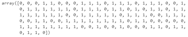
Image 3 — Predicted classes (image by author)
And here are the actual classes (y_test):
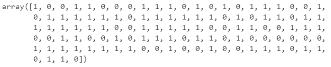
Image 4 — Actual classes (image by author)
As you can see, the arrays are quite similar but have differences in a couple of places. A simple accuracy will tell us the percentage of instances classified correctly:
from sklearn.metrics import accuracy_score

accuracy_score(y_test, preds)
Here’s the corresponding accuracy:
Image 5 — KNN model accuracy (image by author)
Is 93% the best we can get? Unlikely. Let’s explore how you can tweak the value of K and find the optimal one in a range.
K Optimization
It’s highly unlikely that the default K value (3) is the best one. Luckily, it’s easy to do hyperparameter optimization for this simple algorithm. All we have to do is to train the model for some number of K values and select the one where accuracy was the highest.
It’s worth mentioning that only odd numbers should be tested for K values — to avoid potential ties.
The following code snippet evaluates the model for every odd number between 1 and 15:
evals = []

for k in range(1, 16, 2):
    model = KNN(k=k)
    model.fit(X_train, y_train)
    preds = model.predict(X_test)
    accuracy = accuracy_score(y_test, preds)
    evals.append({'k': k, 'accuracy': accuracy})
Let’s visualize the accuracies. The following code snippet makes a plot of K values on the X-axis and their corresponding accuracies on the Y-axis. The optimal one is shown in the title:
evals = pd.DataFrame(evals)
best_k = evals.sort_values(by='accuracy', ascending=False).iloc[0]

plt.figure(figsize=(16, 8))
plt.plot(evals['k'], evals['accuracy'], lw=3, c='#087E8B')
plt.scatter(best_k['k'], best_k['accuracy'], s=200, c='#087E8B')
plt.title(f"K Parameter Optimization, Optimal k = {int(best_k['k'])}", size=20)
plt.xlabel('K', size=14)
plt.ylabel('Accuracy', size=14)
plt.show()
Here are the results:
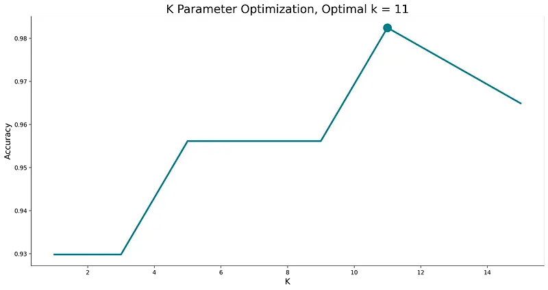
Image 6 — Optimal K value visualization (image by author)
K value of 11 seems to work the best with our dataset. You can now retrain the model having this in mind (model = KNN(k=11).
Let’s compare performance with the Scikit-Learn model next.
Comparison with Scikit-Learn
We want to know if our model is any good, so let’s compare it with something we know works well — a KNeighborsClassifier class from Scikit-Learn.
You can use the following snippet to import the model class, train the model, make predictions, and print the accuracy score:
from sklearn.neighbors import KNeighborsClassifier

knn_model = KNeighborsClassifier()
knn_model.fit(X_train, y_train)
knn_preds = knn_model.predict(X_test)

accuracy_score(y_test, knn_preds)
The corresponding accuracy is shown below:
Image 7 — Scikit-Learn model accuracy (image by author)
As you can see, the model from Scikit-Learn performs roughly the same, at least accuracy-wise. Keep in mind that we didn’t do any tuning here, which would probably bring the accuracy to above 98%.
And that’s all for today. Let’s wrap things up in the next section.
Conclusion
Today you’ve learned how to implement K nearest neighbors in Python entirely from scratch. Does that mean you should ditch the de facto standard machine learning libraries? No, not at all. Let me elaborate.
Just because you can write something from scratch doesn’t mean you should. Still, knowing every detail of how algorithms work is a valuable skill and can help you stand out from every other fit and predict data scientist.
Thanks for reading, and please stay tuned to the blog if you’re interested in more machine learning from scratch articles.
Stay connected
- Sign up for my newsletter
- Subscribe on YouTube
- Connect on LinkedIn