Machine Learning can be easy and intuitive — here’s a complete from-scratch guide to Decision Trees
Decision trees are one of the most intuitive machine learning algorithms used both for classification and regression. After reading, you’ll know how to implement a decision tree classifier entirely from scratch.
This is the fifth of many upcoming from-scratch articles, so stay tuned to the blog if you want to learn more. The links to the previous articles are located at the end of this piece.
The article is structured as follows:
- Introduction to Decision Trees
- Math Behind Decision Trees
- Recursion Crash Course
- From-Scratch Implementation
- Model Evaluation
- Comparison with Scikit-Learn
- Conclusion
You can download the corresponding notebook here.
Introduction to Decision Trees
Decision trees are a non-parametric model used for both regression and classification tasks. The from-scratch implementation will take you some time to fully understand, but the intuition behind the algorithm is quite simple.
Decision trees are constructed from only two elements — nodes and branches. We’ll discuss different types of nodes in a bit. If you decide to follow along, the term recursion shouldn’t feel like a foreign language, as the algorithm is based on this concept. You’ll get a crash course in recursion in a couple of minutes, so don’t sweat it if you’re a bit rusty on the topic.
Let’s take a look at an example decision tree first:
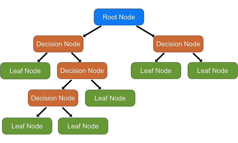
Image 1 — Example decision tree representation with node types (image by author)
As you can see, there are multiple types of nodes:
- Root node— node at the top of the tree. It contains a feature that best splits the data (a single feature that alone classifies the target variable most accurately)
- Decision nodes— nodes where the variables are evaluated. These nodes have arrows pointing to them and away from them
- Leaf nodes— final nodes at which the prediction is made
Depending on the dataset size (both in rows and columns), there are probably thousands to millions of ways the nodes and their conditions can be arranged. So, how do we determine the root node?
How to determine the root node
In a nutshell, we need to check how every input feature classifies the target variable independently. If none of the features alone is 100% correct in the classification, we can consider these features impure.
To further decide which of the impure features is most pure, we can use the Entropy metric. We’ll discuss the formula and the calculations later, but you should remember that the entropy value ranges from 0 (best) to 1 (worst).
The variable with the lowest entropy is then used as a root node.
Training process
To begin training the decision tree classifier, we have to determine the root node. That part has already been discussed.
Then, for every single split, the Information gain metric is calculated. Put simply, it represents an average of all entropy values based on a specific split. We’ll discuss the formula and calculations later, but please remember that the higher the gain is, the better the decision split is.
The algorithm then performs a greedy search — goes over all input features and their unique values, calculates information gain for every combination, and saves the best split feature and threshold for every node.
In this way, the tree is built recursively. The recursion process could go on forever, so we’ll have to specify some exit conditions manually. The most common ones are maximum depth and minimum samples at the node. Both will be discussed later upon implementation.
Prediction process
Once the tree is built, we can make predictions for unseen data by recursively traversing the tree. We can check for the traversal direction (left or right) based on the input data and learned thresholds at each node.
Once the leaf node is reached, the most common value is returned.
And that’s it for the basic theory and intuition behind decision trees. Let’s talk about the math behind the algorithm in the next section.
Math Behind Decision Trees
Decision trees represent much more of a coding challenge than a mathematical one. You’ll only have to implement two formulas for the learning part — entropy and information gain.
Let’s start with entropy. As mentioned earlier, it measures a purity of a split at a node level. Its value ranges from 0 (pure) and 1 (impure).
Here’s the formula for entropy:
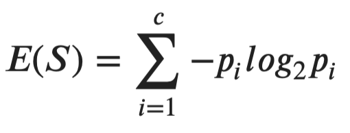
Image 2 — Entropy formula (image by author)
As you can see, it’s a relatively simple equation, so let’s see it in action. Imagine you want to calculate the purity of the following vector:
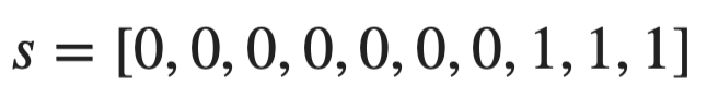
Image 3 — Entropy input (image by author)
To summarize, zeros and ones are the class labels with the following counts:
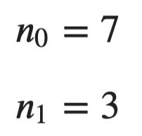
Image 4 — Class distribution summary (image by author)
The entropy calculation is as simple as it can be from this point (rounded to five decimal points):
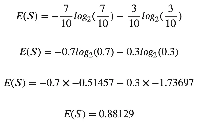
Image 5 — Entropy calculation (image by author)
The result of 0.88 indicates the split is nowhere near pure. Let’s repeat the calculation in Python next. The following code implements the entropy(s) formula and calculates it on the same vector:
import numpy as np
from collections import Counter


def entropy(s):
    counts = np.bincount(s)
    percentages = counts / len(s)

    entropy = 0
    for pct in percentages:
        if pct > 0:
            entropy += pct * np.log2(pct)
    return -entropy

s = [0, 0, 0, 0, 0, 0, 0, 1, 1, 1]
print(f'Entropy: {np.round(entropy(s), 5)}')
The results are shown in the following image:

Image 6 — Entropy calculation in Python (image by author)
As you can see, the results are identical, indicating the formula was implemented correctly.
Let’s take a look at the information gain next. It represents an average of all entropy values based on a specific split. The higher the information gain value, the better the decision split is.
Information gain can be calculated with the following formula:
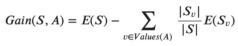
Image 7 — Information gain formula (image by author)
Let’s take a look at an example split and calculate the information gain:
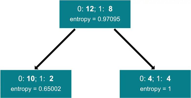
Image 8 — Example split for information gain calculation (image by author)
As you can see, the entropy values were calculated beforehand, so we don’t have to waste time on them. Calculating information gain is now a trivial process:
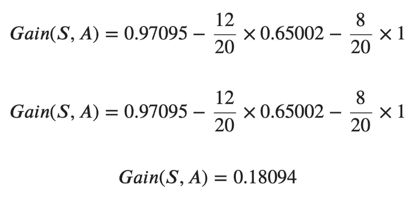
Image 9 — Information gain calculation (image by author)
Let’s implement it in Python next. The following code snippet implements the information_gain() function and calculates it for the previously discussed split:
def information_gain(parent, left_child, right_child):
    num_left = len(left_child) / len(parent)
    num_right = len(right_child) / len(parent)

    gain = entropy(parent) - (num_left * entropy(left_child) + num_right * entropy(right_child))
    return gain

parent = [0, 0, 0, 0, 0, 0, 0, 0, 0, 0, 0, 0, 1, 1, 1, 1, 1, 1, 1, 1]
left_child = [0, 0, 0, 0, 0, 0, 0, 0, 0, 0, 1, 1]
right_child = [0, 0, 0, 0, 1, 1, 1, 1]

print(f'Information gain: {np.round(information_gain(parent, left_child, right_child), 5)}')
The results are shown in the following image:
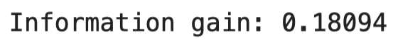
Image 10 — Information gain calculation in Python (image by author)
As you can see, the values match.
And that’s all there is to the math behind decision trees. I’ll repeat — this algorithm is much more challenging to implement in code than to understand mathematically. That’s why you’ll need an additional primer on recursion — coming up next.
Recursion Crash Course
A lot of implementation regarding decision trees boils down to recursion. This section will provide a sneak peek at recursive functions and isn’t by any means a go-to guide to the topic. If this term is new to you, please research it if you want to understand decision trees.
Put simply, a recursive function is a function that calls itself. We don’t want this process going on indefinitely, so the function will need an exit condition. You’ll find it written at the top of the function.
Let’s take a look at the simplest example possible — a recursive function that returns a factorial of an integer:
def factorial(x):
    # Exit condition
    if x == 1:
        return 1
    return x * factorial(x - 1)

print(f'Factorial of 5 is {factorial(5)}')
The results are shown in the following image:
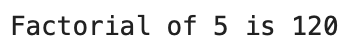
Image 11 — Factorial calculation in Python (image by author)
As you can see, the function calls itself until the entered number isn’t 1. That’s the exit condition of our function.
Recursion is needed in decision tree classifiers to build additional nodes until some exit condition is met. That’s why it’s crucial to understand this concept.
Up next, we’ll implement the classifier. It will require around 200 lines of code (minus the docstrings and comments), so embrace yourself.
From-Scratch Implementation
We’ll need two classes:
Node– implements a single node of a decision treeDecisionTree– implements the algorithm
Let’s start with the Node class. It is here to store the data about the feature, threshold, data going left and right, information gain, and the leaf node value. All are initially set to None. The root and decision nodes will contain values for everything besides the leaf node value, and the leaf node will contain the opposite.
Here’s the code for the class:
class Node:
    '''
    Helper class which implements a single tree node.
    '''
    def __init__(self, feature=None, threshold=None, data_left=None, data_right=None, gain=None, value=None):
        self.feature = feature
        self.threshold = threshold
        self.data_left = data_left
        self.data_right = data_right
        self.gain = gain
        self.value = value
That was the easy part. Let’s implement the classifier next. It will contain a bunch of methods, all of which are discussed below:
__init__()– the constructor, holds values formin_samples_splitandmax_depth. These are hyperparameters. The first one is used to specify a minimum number of samples required to split a node, and the second one specifies a maximum depth of a tree. Both are used in recursive functions as exit conditions_entropy(s)– calculates the impurity of an input vectors_information_gain(parent, left_child, right_child)calculates the information gain value of a split between a parent and two children_best_split(X, y)function calculates the best splitting parameters for input featuresXand a target variabley. It does so by iterating over every column inXand every threshold value in every column to find the optimal split using information gain_build(X, y, depth)function recursively builds a decision tree until stopping criteria is met (hyperparameters in the constructor)fit(X, y)function calls the_build()function and stores the built tree to the constructor_predict(x)function traverses the tree to classify a single instancepredict(X)function applies the_predict()function to every instance in matrixX.
It’s a lot — no arguing there. Take your time to understand every line from the code snippet below. It is well-documented, so the comments should help a bit:
class DecisionTree:
    '''
    Class which implements a decision tree classifier algorithm.
    '''
    def __init__(self, min_samples_split=2, max_depth=5):
        self.min_samples_split = min_samples_split
        self.max_depth = max_depth
        self.root = None

    @staticmethod
    def _entropy(s):
        '''
        Helper function, calculates entropy from an array of integer values.

        :param s: list
        :return: float, entropy value
        '''
        # Convert to integers to avoid runtime errors
        counts = np.bincount(np.array(s, dtype=np.int64))
        # Probabilities of each class label
        percentages = counts / len(s)

        # Caclulate entropy
        entropy = 0
        for pct in percentages:
            if pct > 0:
                entropy += pct * np.log2(pct)
        return -entropy

    def _information_gain(self, parent, left_child, right_child):
        '''
        Helper function, calculates information gain from a parent and two child nodes.

        :param parent: list, the parent node
        :param left_child: list, left child of a parent
        :param right_child: list, right child of a parent
        :return: float, information gain
        '''
        num_left = len(left_child) / len(parent)
        num_right = len(right_child) / len(parent)

        # One-liner which implements the previously discussed formula
        return self._entropy(parent) - (num_left * self._entropy(left_child) + num_right * self._entropy(right_child))

    def _best_split(self, X, y):
        '''
        Helper function, calculates the best split for given features and target

        :param X: np.array, features
        :param y: np.array or list, target
        :return: dict
        '''
        best_split = {}
        best_info_gain = -1
        n_rows, n_cols = X.shape

        # For every dataset feature
        for f_idx in range(n_cols):
            X_curr = X[:, f_idx]
            # For every unique value of that feature
            for threshold in np.unique(X_curr):
                # Construct a dataset and split it to the left and right parts
                # Left part includes records lower or equal to the threshold
                # Right part includes records higher than the threshold
                df = np.concatenate((X, y.reshape(1, -1).T), axis=1)
                df_left = np.array([row for row in df if row[f_idx] <= threshold])
                df_right = np.array([row for row in df if row[f_idx] > threshold])

                # Do the calculation only if there's data in both subsets
                if len(df_left) > 0 and len(df_right) > 0:
                    # Obtain the value of the target variable for subsets
                    y = df[:, -1]
                    y_left = df_left[:, -1]
                    y_right = df_right[:, -1]

                    # Caclulate the information gain and save the split parameters
                    # if the current split if better then the previous best
                    gain = self._information_gain(y, y_left, y_right)
                    if gain > best_info_gain:
                        best_split = {
                            'feature_index': f_idx,
                            'threshold': threshold,
                            'df_left': df_left,
                            'df_right': df_right,
                            'gain': gain
                        }
                        best_info_gain = gain
        return best_split

    def _build(self, X, y, depth=0):
        '''
        Helper recursive function, used to build a decision tree from the input data.

        :param X: np.array, features
        :param y: np.array or list, target
        :param depth: current depth of a tree, used as a stopping criteria
        :return: Node
        '''
        n_rows, n_cols = X.shape

        # Check to see if a node should be leaf node
        if n_rows >= self.min_samples_split and depth <= self.max_depth:
            # Get the best split
            best = self._best_split(X, y)
            # If the split isn't pure
            if best['gain'] > 0:
                # Build a tree on the left
                left = self._build(
                    X=best['df_left'][:, :-1],
                    y=best['df_left'][:, -1],
                    depth=depth + 1
                )
                right = self._build(
                    X=best['df_right'][:, :-1],
                    y=best['df_right'][:, -1],
                    depth=depth + 1
                )
                return Node(
                    feature=best['feature_index'],
                    threshold=best['threshold'],
                    data_left=left,
                    data_right=right,
                    gain=best['gain']
                )
        # Leaf node - value is the most common target value
        return Node(
            value=Counter(y).most_common(1)[0][0]
        )

    def fit(self, X, y):
        '''
        Function used to train a decision tree classifier model.

        :param X: np.array, features
        :param y: np.array or list, target
        :return: None
        '''
        # Call a recursive function to build the tree
        self.root = self._build(X, y)

    def _predict(self, x, tree):
        '''
        Helper recursive function, used to predict a single instance (tree traversal).

        :param x: single observation
        :param tree: built tree
        :return: float, predicted class
        '''
        # Leaf node
        if tree.value != None:
            return tree.value
        feature_value = x[tree.feature]

        # Go to the left
        if feature_value <= tree.threshold:
            return self._predict(x=x, tree=tree.data_left)

        # Go to the right
        if feature_value > tree.threshold:
            return self._predict(x=x, tree=tree.data_right)

    def predict(self, X):
        '''
        Function used to classify new instances.

        :param X: np.array, features
        :return: np.array, predicted classes
        '''
        # Call the _predict() function for every observation
        return [self._predict(x, self.root) for x in X]
You’re not expected to understand every line of code in one sitting. Give it time, go over the code line by line and try to reason why things work. It’s not that difficult once you understand the basic intuition behind the algorithm.
Model Evaluation
Let’s test our classifier next. We’ll use the Iris dataset from Scikit-Learn. The following code snippet loads the dataset and separates it into features (X) and the target (y):
from sklearn.datasets import load_iris

iris = load_iris()

X = iris['data']
y = iris['target']
Let’s split the dataset into training and testing portions next. The following code snippet does just that, in an 80:20 ratio:
from sklearn.model_selection import train_test_split

X_train, X_test, y_train, y_test = train_test_split(X, y, test_size=0.2, random_state=42)
And now let’s do the training. The code snippet below trains the model with default hyperparameters and makes predictions on the test set:
model = DecisionTree()
model.fit(X_train, y_train)
preds = model.predict(X_test)
Let’s take a look at the generated predictions (preds):

Image 12 — Custom decision tree predictions on the test set (image by author)
And now at the actual class labels (y_test):

Image 13 — Test set class labels (image by author)
As you can see, both are identical, indicating a perfectly accurate classifier. You can further evaluate the performance if you want. The code below prints the accuracy score on the test set:
from sklearn.metrics import accuracy_score

accuracy_score(y_test, preds)
As expected, the value of 1.0 would get printed. Don’t let this fool you – the Iris dataset is incredibly easy to classify correctly, especially if you get a good “random” test set. Still, let’s compare our classifier to the one built into Scikit-Learn.
Comparison with Scikit-Learn
We want to know if our model is any good, so let’s compare it with something we know works well — a DecisionTreeClassifier class from Scikit-Learn.
You can use the following snippet to import the model class, train the model, make predictions, and print the accuracy score:
from sklearn.tree import DecisionTreeClassifier

sk_model = DecisionTreeClassifier()
sk_model.fit(X_train, y_train)
sk_preds = sk_model.predict(X_test)

accuracy_score(y_test, sk_preds)
As you would expect, we get a perfect accuracy score of 1.0.
And that’s all for today. Let’s wrap things up in the next section.
Conclusion
This was one of the most challenging articles I have ever written. It took around a week to get everything right and to make the code as understandable as possible. Naturally, it will take you at least a couple of readings to understand the topic altogether. Feel free to explore additional resources, as it will further advance your understanding.
You now know how to implement the Decision tree classifier algorithm from scratch. Does that mean you should ditch the de facto standard machine learning libraries? No, not at all. Let me elaborate.
Just because you can write something from scratch doesn’t mean you should. Still, knowing every detail of how algorithms work is a valuable skill and can help you stand out from every other fit and predict data scientist.
Thanks for reading, and please stay tuned to the blog if you’re interested in more machine learning from scratch articles.
Stay connected
- Sign up for my newsletter
- Subscribe on YouTube
- Connect on LinkedIn