
In-database machine learning? It’s easier than you think
It seems like everybody knows how to train predictive models in languages like Python, R, and Julia. But what about SQL? How can you leverage the power of a well-known database language for machine learning?
SQL has been around for decades, but still isn’t recognized as a language for machine learning. Sure, I’d pick Python any day of the week, but sometimes in-database machine learning is the only option.
We’ll use Oracle Cloud for this article. It’s free, so please register and create an instance of the OLTP database (Version 19c, has 0.2TB of storage). Once done, establish a connection through the SQL Developer Web— or any other tool.
We’ll use a slightly modified version of a well-known Housing prices dataset — you can download it here. I’ve chosen this dataset because it doesn’t require any extensive preparation, so the focus can immediately be shifted to predictive modeling.
The article is structured as follows:
- Dataset loading and preparation
- Model settings
- Model training and evaluation
- Conclusion
Dataset loading and preparation
If you are following along, I hope you’ve downloaded the datasetalready. You need to load it into the database with a tool of your choice — I’m using SQL Developer Web, a free tool provided by Oracle Cloud.
The loading process is straightforward — click on the upload button, choose the CSV file, and click Next a couple of time:

Image 1 — Dataset loading with Oracle SQL Developer Web (image by author)
Mine is now stored in the housingprices table. Here’s how the first couple of rows look like:
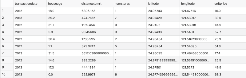
Image 2 — First 10 rows of the loaded dataset (image by author)
Oracle Machine Learning (OML) is a bit strange when it comes to creating models. Your data table must contain a column with an ID — numbers generated from a sequence. Our dataset doesn’t have that by default, so let’s add it manually:
CREATE SEQUENCE seq_housingprices;
ALTER TABLE housingprices ADD (
    row_id INTEGER DEFAULT seq_housingprices.NEXTVAL
);
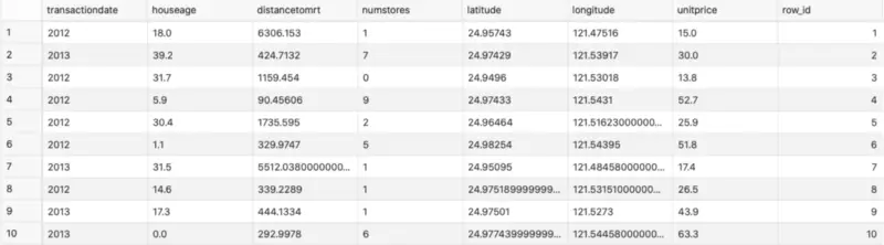
Image 3 — Added a column for row ID (image by author)
There’s only one thing left to do in this section: the train/test split. In SQL, that’s done by creating two views. The first view has 75% of the data randomly sampled, and the second one has the remaining 25%. The percentages were chosen arbitrarily:
BEGIN
    EXECUTE IMMEDIATE
        'CREATE OR REPLACE VIEW
        	housing_train_data AS
        	SELECT * FROM housingprices
        	SAMPLE (75) SEED (42)';
    EXECUTE IMMEDIATE
        'CREATE OR REPLACE VIEW
        	housing_test_data AS
        	SELECT * FROM housingprices
        	MINUS
        	SELECT * FROM housing_train_data';
END;
/
We now have two views created —housing_train_data for training and housing_test_data for testing. There’s still one thing left to do before model training: to specify settings for the model. Let’s do that in the next section.
Model settings
Oracle uses this settings table style for training predictive models. The settings table is made of two columns — one for the name and the other for the value.
Here’s how to create the table:
CREATE TABLE housing_model_settings(
	setting_name VARCHAR2(30),
  	setting_value VARCHAR2(4000)
);
The following information will be stored in this table:
- Type of model — let’s use a Generalized Linear Model (GLM)
- Diagnostics table name — for model statistics
- Data preparation technique — let’s go with the automatic
- Feature selection — disabled or enabled, let’s go with enabled
- Feature generation — same as with feature selection
Yes, you are reading this right — all of that is done automatically without the need for your assistance. Let’s fill the settings table next:
BEGIN
    INSERT INTO housing_model_settings VALUES(DBMS_DATA_MINING.ALGO_NAME, DBMS_DATA_MINING.ALGO_GENERALIZED_LINEAR_MODEL);

    -- Row diagnostic statistics
    INSERT INTO housing_model_settings VALUES(DBMS_DATA_MINING.GLMS_DIAGNOSTICS_TABLE_NAME, 'GLMS_HOUSING_DIAG');

    -- Auto data preparation
    INSERT INTO housing_model_settings VALUES(DBMS_DATA_MINING.PREP_AUTO, DBMS_DATA_MINING.PREP_AUTO_ON);

    -- Feature selection
    INSERT INTO housing_model_settings VALUES(DBMS_DATA_MINING.GLMS_FTR_SELECTION, DBMS_DATA_MINING.GLMS_FTR_SELECTION_ENABLE);

    -- Feature generation
    INSERT INTO housing_model_settings VALUES(DBMS_DATA_MINING.GLMS_FTR_GENERATION, DBMS_DATA_MINING.GLMS_FTR_GENERATION_ENABLE);
END;
/
Here’s how the table looks like:
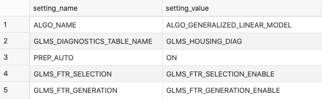
Image 4 — Model settings table (image by author)
And that’s it! Let’s continue with the model training.
Model training and validation
The model training boils down to a single procedure call. Here’s the code:
BEGIN
  	DBMS_DATA_MINING.CREATE_MODEL(
  		  model_name          => 'GLMR_Regression_Housing',
        mining_function     => DBMS_DATA_MINING.REGRESSION,
        data_table_name     => 'housing_train_data',
      	case_id_column_name => 'row_id',
        target_column_name  => 'unitprice',
        settings_table_name => 'housing_model_settings'
  	);
END;
/
As you can see, you need to name your model first. The name GLMR_Regression_Housing is entirely arbitrary. After a second or so, the model is trained. Don’t get scared with the number of tables Oracle creates. Those are required for a model to work properly.
Next, let’s take a peek at the model performance on the train set. It can be obtained with the following query:
SELECT *
	FROM TABLE(DBMS_DATA_MINING.GET_MODEL_DETAILS_GLOBAL('GLMR_Regression_Housing'))
ORDER BY global_detail_name;
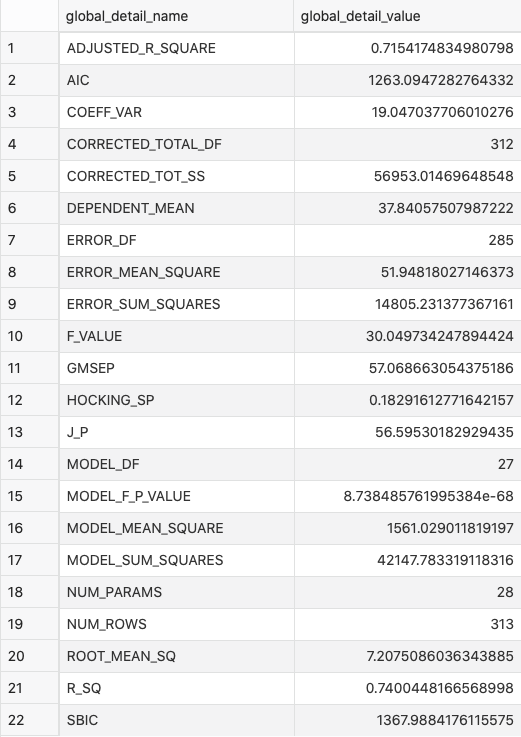
Image 5 — Model performance on the train set (image by author)
On average, the model is wrong by 7.2 units of the price, and it captures just north of 70% of the variance.
Let’s take a look at the most significant features next. The feature can be classified as significant for prediction if its P-value is somewhere near 0 (less than 0.05 will do). Here’s the query:
SELECT feature_expression, coefficient, p_value
	FROM TABLE(DBMS_DATA_MINING.GET_MODEL_DETAILS_GLM('GLMR_Regression_Housing'))
ORDER BY p_value DESC;
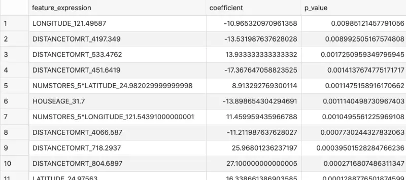
Image 6 — Feature importances (image by author)
As you can see, these features weren’t present initially in the dataset but were created automatically by Oracle’s feature generator.
Finally, let’s apply this model to the test set:
BEGIN
    DBMS_DATA_MINING.APPLY(
        'GLMR_Regression_Housing',
        'housing_test_data',
        'row_id',
        'housing_test_predictions'
    );
END;
/
The results are stored in the housing_test_predictions table:
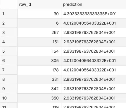
Image 7 — Predictions on the test set (image by author)
Don’t know what’s the deal with the scientific notation, but it’s good enough for further evaluation. I’ll leave it up to you, as you only need to create a UNION between the housing_test_data view and the housing_test_predictions table to see how good are the results.
Parting words
Machine learning isn’t a Python or R specific thing anymore. Adoption in SQL isn’t the most intuitive for a data scientist, and the documentation is awful, but in-database ML provides an excellent way for business users to get in touch with predictive modeling.
Feel free to leave any thoughts in the comment section below.