Classification fundamentals in R — code included
Our little journey to machine learning with R continues! Today’s topic is logistic regression — as an introduction to machine learning classification tasks. We’ll cover data preparation, modeling, and evaluation of the well-known Titanic dataset.
This article is structured as follows:
- Intro to logistic regression
- Dataset introduction and loading
- Data preparation
- Model training and evaluation
- Conclusion
You can download the source code here. That’s it for the introduction section — we have many things to cover, so let’s jump right to it.
Intro to logistic regression
Logistic regression is a great introductory algorithm for binary classification (two class values) borrowed from the field of statistics. The algorithm got the name from its underlying mechanism — the logistic function (sometimes called the sigmoid function).
The logistic function is an S-shaped function developed in statistics, and it takes any real-valued number and maps it to a value between 0 and 1. That’s just what we need for binary classification, as we can set the threshold at 0.5 and make predictions according to the output of the logistic function.
Here’s how the logistic function looks like:
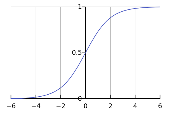
Image by author
In case you’re interested, below is the equation for the logistic function. Remember — it takes any real-valued number and transforms it to a value between 0 and 1.

Image by author
And that’s quite enough for the theory. I repeat — this article’s aim isn’t to cover the theory, as there’s a plethora of theoretical articles/books out there. It’s a pure hands-on piece.
Dataset introduction and loading
Okay, now we have a basic logistic regression understanding under our belt, and we can begin with the coding portion. We’ll use the Titanic dataset, as mentioned previously. You don’t have to download it, as _R_does that for us.
Here’s the snippet for library imports and dataset loading:
library(dplyr)
library(stringr)
library(caTools)
library(caret)
df <- read.csv('https://raw.githubusercontent.com/datasciencedojo/datasets/master/titanic.csv')
And here’s how the first couple of rows look like:
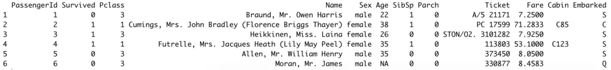
Image by author
Awesome! The dataset requires a bit of preparation to get it to a ml-ready format, so that’s what we’ll do next.
Data preparation
There are a couple of essential things we have to do:
- Extract titles from the Name attribute
- Remap extracted titles as usual/unusual
- Convert Cabin attribute to binary — HasCabin
- Remove unnecessary attributes
This snippet from Kaggle helped a lot with title extraction and remapping, with slight modifications. Other points are relatively straightforward, as the following snippet shows:
maleNobleTitles <- c('Capt', 'Col', 'Don', 'Dr', 'Jonkheer', 'Major', 'Rev', 'Sir')
femaleNobleTitles <- c('Lady', 'Mlle', 'Mme', 'Ms', 'the Countess')

df$Title <- str_sub(df$Name, str_locate(df$Name, ',')[ , 1] + 2, str_locate(df$Name, '\\.')[ , 1] - 1)
df$Title[df$Title %in% maleNobleTitles] <- 'MaleNoble'
df$Title[df$Title %in% femaleNobleTitles] <- 'FemaleNoble'
df$HasCabin <- ifelse(df$Cabin == '', 0, 1)
df <- df %>% select(-PassengerId, -Name, -Ticket, -Cabin)
We essentially created two arrays for noble titles, one for males and one for females, extracted the title to the Title column, and replaced noble titles with the expressions ‘MaleNoble’ and ‘FemaleNoble’.
Further, the ifelse function helped make the HasCabin attribute, which has a value of 1 if the value for Cabin is not empty and 0 otherwise. Finally, we’ve kept only the features that are relevant for analysis.
Here’s how the dataset looks now:
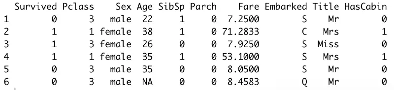
Image by author
Awesome! Let’s deal with missing values next.
Handling missing data
The following line of code prints out how many missing values there are per attribute:
lapply(df, function(x) { length(which(is.na(x))) })
The attribute Age is the only one that contains missing values. As this article covers machine learning and not data preparation, we’ll perform the imputation with a simple mean. Here’s the snippet:
df$Age <- ifelse(is.na(df$Age), mean(df$Age, na.rm=TRUE), df$Age)
And that’s it for the imputation. There’s only one thing left to do, preparation-wise.
Factor conversion
We have a bunch of categorical attributes in our dataset. R provides a simple factor() function that converts categorical attributes to an algorithm-understandable format.
Here’s the structure of our dataset before the transformation:
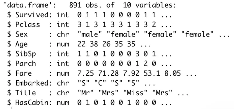
Image by author
And here’s the code snippet to perform the transformation:
df$Survived <- factor(df$Survived)
df$Pclass <- factor(df$Pclass)
df$Sex <- factor(df$Sex)
df$SibSp <- factor(df$SibSp)
df$Parch <- factor(df$Parch)
df$Embarked <- factor(df$Embarked)
df$Title <- factor(df$Title)
df$HasCabin <- factor(df$HasCabin)
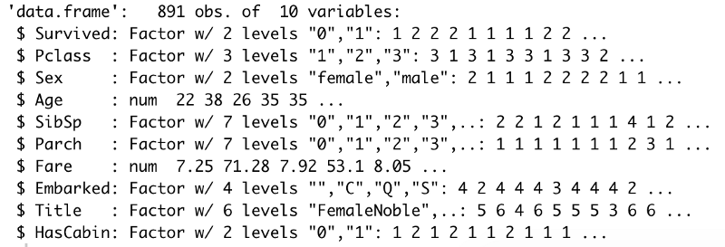
Image by author
The data preparation part is finished, and we can now proceed with the modeling.
Model training and evaluation
Before the actual model training, we need to split our dataset on the training and testing subset. Doing so ensures we have a subset of data to evaluate on, and know how good the model is. Here’s the code:
set.seed(42)
sampleSplit <- sample.split(Y=df$Survived, SplitRatio=0.7)
trainSet <- subset(x=df, sampleSplit==TRUE)
testSet <- subset(x=df, sampleSplit==FALSE)
The above code divides the original dataset into 70:30 subsets. We’ll train on the majority (70%), and evaluate on the rest.
We can now train the model with the function. We’ll use all of the attributes, indicated by the dot, and the column is the target variable.
model <- glm(Survived ~ ., family=binomial(link='logit'), data=trainSet)
And that’s it — we have successfully trained the model. Let’s see how it performed by calling the summary() function on it:
summary(model)
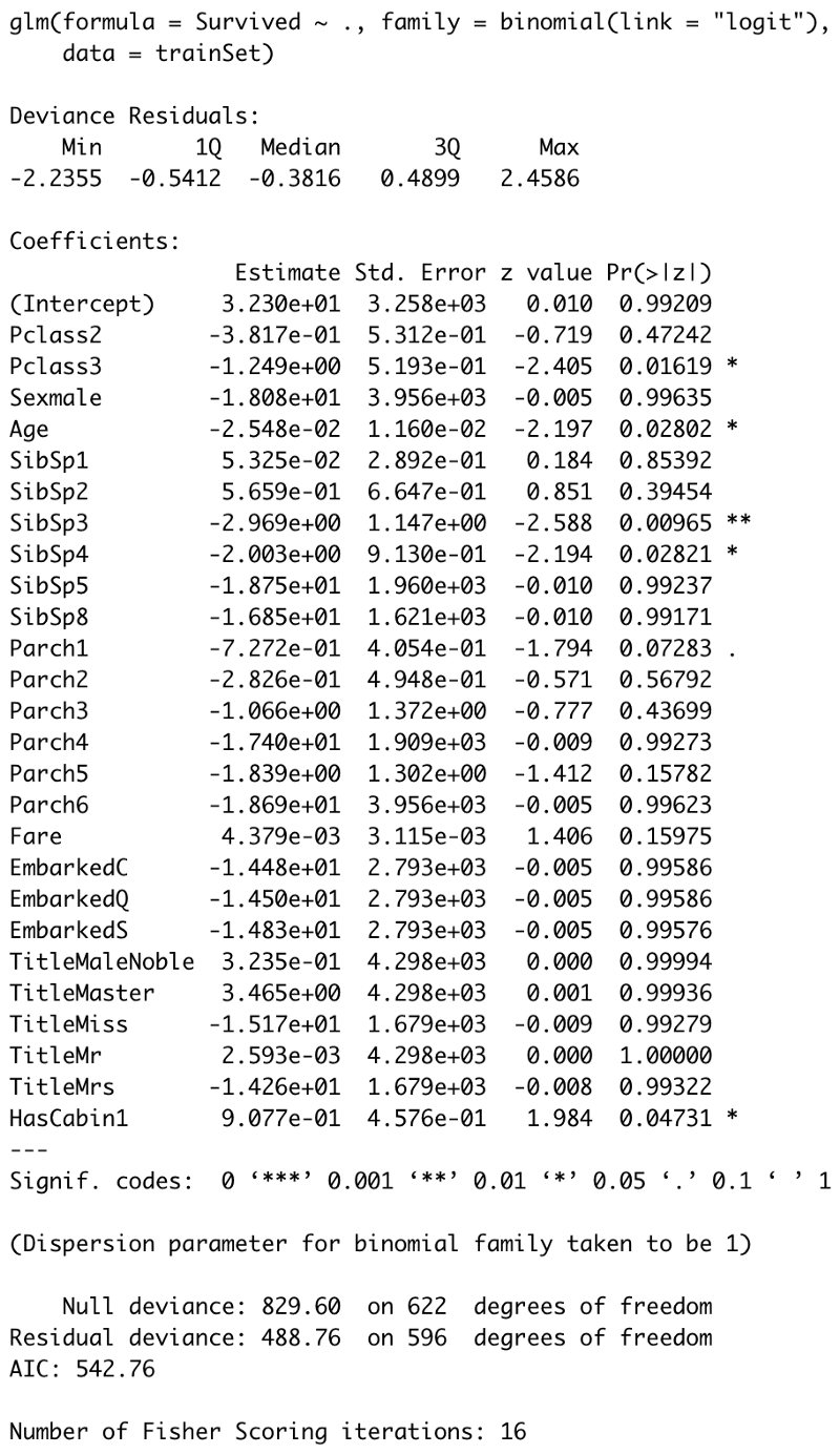
Image by author
The most exciting thing here is the P-values, displayed in the **Pr(>|t|)**column. Those values indicate the probability of a variable not being important for prediction. It’s common to use a 5% significance threshold, so if a P-value is 0.05 or below, we can say there’s a low chance for it not being significant for the analysis.
As we can see, the most significant attributes/attribute subsets are Pclass3, __ Age, __ SibSp3, __ SibSp4 , and HasCabin1.
We now have some more info on our model — we know the most important factors to decide if a passenger survived the Titanic accident. Now we can move on the evaluation of previously unseen data — test set.
We’ve kept this subset untouched deliberately, just for model evaluation. To start, we’ll need to calculate the prediction probabilities and predicted classes on top of those probabilities. We’ll set 0.5 as a threshold — if the chance of surviving is less than 0.5, we’ll say the passenger didn’t survive the accident. Here’s the code:
probabs <- predict(model, testSet, type='response')
preds <- ifelse(probabs > 0.5, 1, 0)
It’s now easy to build on top of that. The go-to approach for classification tasks is to make a confusion matrix — a 2×2 matrix showing correct classification on the first and fourth element, and incorrect classification on the second and third element (reading left to right, top to bottom). Here’s how to obtain it through code:
confusionMatrix(factor(preds), factor(testSet$Survived))
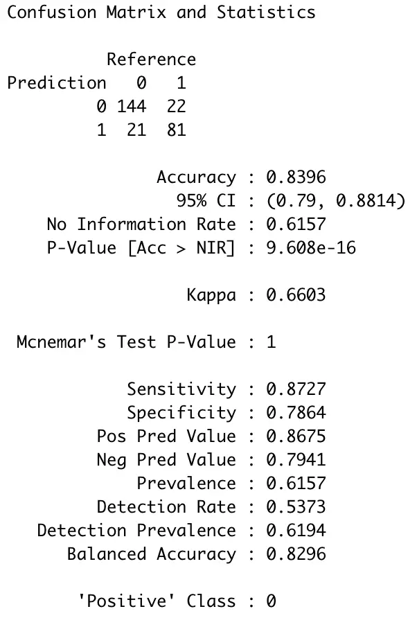
Image by author
So, overall, our model is correct in roughly 84% of the test cases — not too bad for a couple of minutes of work. Let’s wrap things up in the next section.
Before you go
We’ve covered the most basic regression and classification machine learning algorithms thus far. It was quite a tedious process, I know, but necessary to create foundations for what’s coming later — more complex algorithms and optimization.
The next article in the series on KNN is coming in a couple of days, so stay tuned.
Thanks for reading.