There’s a lot of hype behind the new Apple M1 chip. So far, it’s proven to be superior to anything Intel has offered. But what does this mean for deep learning? That’s what you’ll find out today.
The new M1 chip isn’t just a CPU. On the MacBook Pro, it consists of 8 core CPU, 8 core GPU, and 16 core neural engine, among other things. Both the processor and the GPU are far superior to the previous-generation Intel configurations.
I’ve already demonstrated how fast the M1 chip is for regular data science tasks, but what about deep learning?
Short answer — yes, there are some improvements in this department, but are Macs now better than, let’s say, Google Colab? Keep in mind, Colab is an entirely free option.
The article is structured as follows:
- CPU and GPU benchmark
- Performance test — MNIST
- Performance test — Fashion MNIST
- Performance test — CIFAR-10
- Conclusion
Important notes
Not all data science libraries are compatible with the new M1 chip yet. Getting TensorFlow (version 2.4) to work properly is easier said than done.
You can refer to this link to download the .whl files for TensorFlow and it’s dependencies. This is only for macOS 11.0 and above, so keep that in mind.
The test you’ll see aren’t “scientific” in any way, shape or form. They only compare the average training time per epoch.
CPU and GPU benchmark
Let’s start with the basic CPU and GPU benchmarks first. The comparison is made between the new MacBook Pro with the M1 chip and the base model (Intel) from 2019. Geekbench 5 was used for the tests, and you can see the results below:

Image 1 — Geekbench 5 results (Intel MBP vs. M1 MBP) (image by author)
The results speak for themselves. M1 chip demolished Intel chip in my 2019 Mac. So far, things look promising.
Performance test — MNIST
The MNIST dataset is something like a “hello world” of deep learning. It comes built-in with TensorFlow, making it that much easier to test.
The following script trains a neural network classifier for ten epochs on the MNIST dataset. If you’re on an M1 Mac, uncomment the mlcompute lines, as these will make things run a bit faster:
import tensorflow as tf
from tensorflow.keras import datasets, layers, models

(train_images, train_labels), (test_images, test_labels) = datasets.mnist.load_data()
train_images, test_images = train_images / 255.0, test_images / 255.0

# ONLY ON THE MAC
# from tensorflow.python.compiler.mlcompute import mlcompute
# mlcompute.set_mlc_device(device_name='gpu')

model = models.Sequential([
    layers.Flatten(input_shape=(28, 28)),
    layers.Dense(128, activation='relu'),
    layers.Dense(64, activation='relu'),
    layers.Dense(10)
])
model.compile(
    optimizer='adam',
    loss=tf.keras.losses.SparseCategoricalCrossentropy(from_logits=True),
    metrics=['accuracy']
)
history = model.fit(
    train_images,
    train_labels,
    epochs=10,
    validation_data=(test_images, test_labels)
)
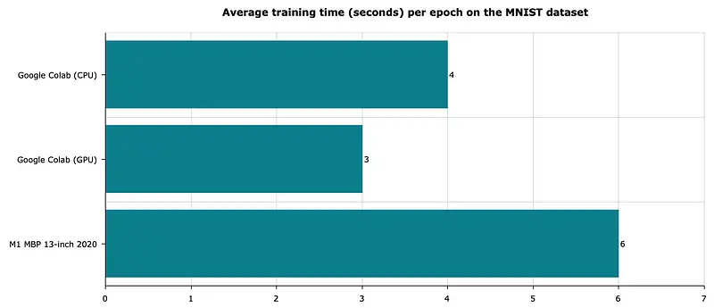
The above script was executed on an M1 MBP and Google Colab (both CPU and GPU). You can see the runtime comparisons below:

Image 2 — MNIST model average training times (image by author)
The results are somewhat disappointing for a new Mac. Colab outperformed it in both CPU and GPU runtimes. Keep in mind that results may vary, as there’s no guarantee of the runtime environment in Colab.
Performance test — Fashion MNIST
This dataset is quite similar to the regular MNIST, but is contains pieces of clothing instead of handwritten digits. Because of that, you can use the identical neural network architecture for the training:
import tensorflow as tf
from tensorflow.keras import datasets, layers, models

(train_images, train_labels), (test_images, test_labels) = datasets.fashion_mnist.load_data()
train_images, test_images = train_images / 255.0, test_images / 255.0

# ONLY ON THE MAC
# from tensorflow.python.compiler.mlcompute import mlcompute
# mlcompute.set_mlc_device(device_name='gpu')

model = models.Sequential([
    layers.Flatten(input_shape=(28, 28)),
    layers.Dense(128, activation='relu'),
    layers.Dense(64, activation='relu'),
    layers.Dense(10)
])
model.compile(
    optimizer='adam',
    loss=tf.keras.losses.SparseCategoricalCrossentropy(from_logits=True),
    metrics=['accuracy']
)
history = model.fit(
    train_images,
    train_labels,
    epochs=10,
    validation_data=(test_images, test_labels)
)
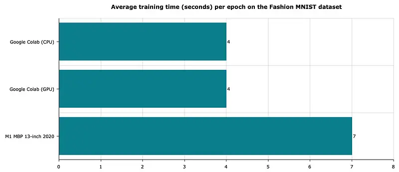
As you can see, the only thing that’s changed here is the function used to load the dataset. The runtime results for the same environments are shown below:

Image 3 — Fashion MNIST model average training times (image by author)
Once again, we get similar results. It’s expected, as this dataset is quite similar to MNIST.
But what will happen if we introduce a more complex dataset and neural network architecture?
Performance test — CIFAR-10
CIFAR-10 also falls into the category of “hello world” deep learning datasets. It contains 60K images from ten different categories, such as airplanes, birds, cats, dogs, ships, trucks, etc.
The images are of size 32x32x3, which makes them difficult to classify even for humans in some cases. The script below trains a classifier model by using three convolutional layers:
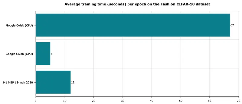
Let’s see how convolutional layers and more complex architecture affects the runtime:

Image 4 — CIFAR-10 model average training times (image by author)
import tensorflow as tf
from tensorflow.keras import datasets, layers, models

(train_images, train_labels), (test_images, test_labels) = datasets.cifar10.load_data()
train_images, test_images = train_images / 255.0, test_images / 255.0

# ONLY ON THE MAC
# from tensorflow.python.compiler.mlcompute import mlcompute
# mlcompute.set_mlc_device(device_name='gpu')

model = models.Sequential()
model.add(layers.Conv2D(32, (3, 3), activation='relu', input_shape=(32, 32, 3)))
model.add(layers.MaxPooling2D((2, 2)))
model.add(layers.Conv2D(64, (3, 3), activation='relu'))
model.add(layers.MaxPooling2D((2, 2)))
model.add(layers.Conv2D(64, (3, 3), activation='relu'))
model.add(layers.Flatten())
model.add(layers.Dense(64, activation='relu'))
model.add(layers.Dense(10))

model.compile(
    optimizer='adam',
    loss=tf.keras.losses.SparseCategoricalCrossentropy(from_logits=True),
    metrics=['accuracy']
)
history = model.fit(
    train_images,
    train_labels,
    epochs=10,
    validation_data=(test_images, test_labels)
)
As you can see, the CPU environment in Colab comes nowhere close to the GPU and M1 environments. The Colab GPU environment is still around 2x faster than Apple’s M1, similar to the previous two tests.
Conclusion
I love every bit of the new M1 chip and everything that comes with it — better performance, no overheating, and better battery life. Still, it’s a difficult laptop to recommend if you’re into deep learning.
Sure, there’s around 2x improvement in M1 than my other Intel-based Mac, but these still aren’t machines made for deep learning. Don’t get me wrong, you can use the MBP for any basic deep learning tasks, but there are better machines in the same price range if you’ll do deep learning daily.
This article covered deep learning only on simple datasets. The next one will compare the M1 chip with Colab on more demanding tasks — such as transfer learning.
Thanks for reading.
Stay connected
- Sign up for my newsletter
- Subscribe on YouTube
- Connect on LinkedIn

