
Black-box models aren’t cool anymore. It’s easy to build great models nowadays, but what’s going on inside? That’s what Explainable AI and LIME try to uncover.
Knowing why the model makes predictions the way it does is essential for tweaking. Just think about it — if you don’t know what’s going on inside, how the hell will you improve it?
Today we also want to train the model ASAP and focus on interpretation. Because of that, the identical dataset and modeling process is used.
After reading this article, you shouldn’t have any problems with explainable machine learning. Interpreting models and the importance of each predictor should become second nature.
What is LIME?
The acronym LIME stands for Local Interpretable Model-agnostic Explanations. The project is about explaining what machine learning models are doing (source). LIME supports explanations for tabular models, text classifiers, and image classifiers (currently).
To install LIME, execute the following line from the Terminal:pip install lime
In a nutshell, LIME is used to explain predictions of your machine learning model. The explanations should help you to understand why the model behaves the way it does. If the model isn’t behaving as expected, there’s a good chance you did something wrong in the data preparation phase.
You’ll now train a simple model and then begin with the interpretations.
Model training
You can’t interpret a model before you train it, so that’s the first step. The Wine quality dataset is easy to train on and comes with a bunch of interpretable features. Here’s how to load it into Python:
import numpy as np
import pandas as pd

wine = pd.read_csv('wine.csv')
wine.head()
The first couple of rows look like this:
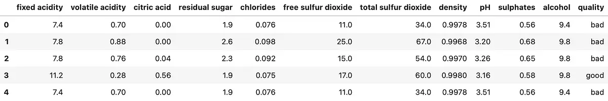
Image 1 — Wine quality dataset head (image by author)
All attributes are numeric, and there are no missing values, so you can cross data preparation from the list.
Train/Test split is the next step. The column quality is the target variable, with possible values of good and bad. Set the random_state parameter to 42 if you want to get the same split:
from sklearn.model_selection import train_test_split

X = wine.drop('quality', axis=1)
y = wine['quality']

X_train, X_test, y_train, y_test = train_test_split(
    X, y, test_size=0.2, random_state=42
)
Model training is the only thing left to do. RandomForestClassifier from ScikitLearn will do the job, and you’ll have to fit it on the training set. You’ll get an 80% accurate classifier out of the box (score):
from sklearn.ensemble import RandomForestClassifier

model = RandomForestClassifier(random_state=42)
model.fit(X_train, y_train)
score = model.score(X_test, y_test)
And that’s all you need to start with model interpretation. You’ll learn how in the next section.
Model interpretation
To start explaining the model, you first need to import the LIME library and create a tabular explainer object. It expects the following parameters:
training_data– our training data generated with train/test split. It must be in a Numpy array format.feature_names– column names from the training setclass_names– distinct classes from the target variablemode– type of problem you’re solving (classification in this case)
Here’s the code:
import lime
from lime import lime_tabular

explainer = lime_tabular.LimeTabularExplainer(
    training_data=np.array(X_train),
    feature_names=X_train.columns,
    class_names=['bad', 'good'],
    mode='classification'
)
And that’s it — you can start interpreting! A bad wine comes in first. The second row of the test set represents wine classified as bad. You can call the explain_instance function of the explainer object to, well, explain the prediction. The following parameters are required:
data_row– a single observation from the datasetpredict_fn– a function used to make predictions. Thepredict_probafrom the model is a great option because it shows probabilities
Here’s the code:
exp = explainer.explain_instance(
    data_row=X_test.iloc[1],
    predict_fn=model.predict_proba
)

exp.show_in_notebook(show_table=True)
The show_in_notebook function shows the prediction interpretation in the notebook environment:
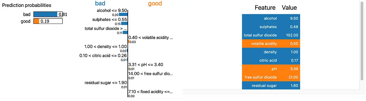
Image 2 — LIME interpretation for a bad wine (image by author)
The model is 81% confident this is a bad wine. The values of alcohol, sulphates, and total sulfur dioxide increase wine’s chance to be classified as bad. The volatile acidity is the only one that decreases it.
Let’s take a look at a good wine next. You can find one at the fifth row of the test set:
exp = explainer.explain_instance(
    data_row=X_test.iloc[4],
    predict_fn=model.predict_proba
)

exp.show_in_notebook(show_table=True)
Here’s the corresponding interpretation:
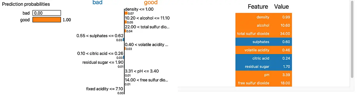
Image 3 — LIME interpretation for a good wine (image by author)
Now that’s the wine I’d like to try. The model is 100% confident it’s a good wine, and the top three predictors show it.
That’s how LIME works in a nutshell. There are different visualizations available, and you are not limited to interpreting only a single instance, but this is enough to get you started. Let’s wrap things up in the next section.
Conclusion
Interpreting machine learning models is simple. It provides you with a great way of explaining what’s going on below the surface to non-technical folks. You don’t have to worry about data visualization, as the LIME library handles that for you.
This article should serve you as a basis for more advanced interpretations and visualizations. You can always learn further on your own.
What are your thoughts on LIME? Do you want to see a comparison between LIME and SHAP? Please let me know.
Learn More
- Python If-Else Statement in One Line - Ternary Operator Explained
- Python Structural Pattern Matching - Top 3 Use Cases to Get You Started
- Dask Delayed - How to Parallelize Your Python Code With Ease
Stay connected
- Sign up for my newsletter
- Subscribe on YouTube
- Connect on LinkedIn