From data gathering and preparation to model training and evaluation — Source code included
Deep learning is everywhere. From sales forecasting to segmenting skin diseases on image data — there’s nothing deep learning algorithms can’t do, given quality data.
If deep learning and TensorFlow are new to you, you’re in the right place. This article will show you the entire process of building a classification model on tabular data. You’ll go from data gathering and preparation to training and evaluating neural network models in just one sitting. Let’s start.
You’ll need TensorFlow 2+, Numpy, Pandas, Matplotlib, and Scikit-Learn installed to follow along.
Don’t feel like reading? Watch my video instead:
You can download the source code on GitHub.
Dataset used
Let’s avoid unnecessary headaches and stick to simple datasets. The wine quality dataset from Kaggle will be good enough for today:

Image 1 — Wine quality dataset from Kaggle (image by author)
The dataset is mostly clean, but isn’t designed for binary classification by default (good/bad wine). Instead, the wines are rated on a scale. We’ll address that later.
Download it and extract the CSV somewhere on your machine, and open up JupyterLab. You’re free to use any other IDE, but all the screenshots below will be from Jupyter.
Data preparation and exploration
The first step is to import Numpy and Pandas, and then to import the dataset. The following snippet does that and also prints a random sample of five rows:
import numpy as np
import pandas as pd


df = pd.read_csv('data/winequalityN.csv')
df.sample(5)
Here’s how the dataset looks like:

Image 2 — Wine quality dataset (image by author)
It’s mostly clean, but there’s still some work to do.
Basic preparation
The dataset has some missing values, but the number isn’t significant, as there are 6497 rows in total:
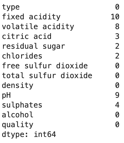
Image 3 — Missing value counts (image by author)
Run the following code to get rid of them:
df = df.dropna()
The only non-numerical feature is type. It can be either white (4870 rows) or red (1593) rows. The following snippet converts this feature to a binary one called is_white_wine, where the value is 1 if type is white and 0 otherwise:
df['is_white_wine'] = [
    1 if typ == 'white' else 0 for typ in df['type']]
df.drop('type', axis=1, inplace=True)
All features are numeric now, and there’s only one thing left to do — make the target variable (quality) binary.
Converting to a binary classification problem
The wines are graded from 3 to 9, assuming higher is better. Here are the value counts:
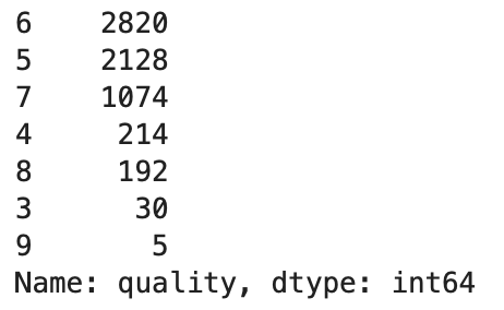
Image 4 — Target variable value counts (image by author)
To keep things extra simple, we’ll convert it into a binary variable. We’ll classify any wine with a grade of 6 and above as good (1), and all other wines as bad (0). Here’s the code:
df['is_good_wine'] = [
    1 if quality >= 6 else 0 for quality in df['quality']
]
df.drop('quality', axis=1, inplace=True)

df.head()
And here’s how the dataset looks like now:

Image 5 — Dataset after preparation (image by author)
You now have 4091 good wines and 2372 bad wines. The classes are imbalanced, but we can work with that. Let’s split the dataset into training and testing sets next.
Train/test split
We’ll stick to a standard 80:20 split. Here’s the code:
from sklearn.model_selection import train_test_split


X = df.drop('is_good_wine', axis=1)
y = df['is_good_wine']

X_train, X_test, y_train, y_test = train_test_split(
    X, y,
    test_size=0.2, random_state=42
)
You now have 5170 rows in the training set and 1293 rows in the testing set. It should be enough to train a somewhat decent neural network model. Let’s scale the data before we start the training.
Data scaling
Features like sulphates and citric acid have values close to zero, while total sulfur dioxide is in hundreds. You’ll confuse the neural network if you leave them as such, as it will think a feature on a higher scale is more important.
That’s where scaling comes into play. We’ll use StandardScaler from Scikit-Learn to fit and transform the training data and to apply the transformation to the testing data:
from sklearn.preprocessing import StandardScaler


scaler = StandardScaler()
X_train_scaled = scaler.fit_transform(X_train)
X_test_scaled = scaler.transform(X_test)
Here’s how the first three scaled rows look like:

Image 6 — Scaled training set (image by author)
The value range is much tighter now, so a neural network should do a better job. Let’s train the model and see if we can get something decent.
Training a classification model with TensorFlow
You’ll need to keep a couple of things in mind when training a binary classification model:
- Output layer structure— You’ll want to have one neuron activated with a sigmoid function. This will output a probability you can then assign to either a good wine (P > 0.5) or a bad wine (P <= 0.5).
- Loss function— Binary cross-entropy is the one to go with. Don’t mistake it for categorical cross-entropy.
- Class balance— Are the classes in the target variable balanced? In other words, do you have roughly the same number of good and bad wines? If not, accuracy might not be the best evaluation metric. We’ll also use precision and recall.
Let’s define a neural network architecture next, having the above three points in mind.
Defining a neural network architecture
I’ve chosen this architecture entirely at random, so feel free to adjust it. The model goes from 12 input features to the first hidden layer of 128 neurons, followed by two additional hidden layers of 256 neurons. There’s a 1-neuron output layer at the end. Hidden layers use ReLU as the activation function, and the output layer uses Sigmoid.
Here’s the code:
import tensorflow as tf
tf.random.set_seed(42)


model = tf.keras.Sequential([
    tf.keras.layers.Dense(128, activation='relu'),
    tf.keras.layers.Dense(256, activation='relu'),
    tf.keras.layers.Dense(256, activation='relu'),
    tf.keras.layers.Dense(1, activation='sigmoid')
])

model.compile(
    loss=tf.keras.losses.binary_crossentropy,
    optimizer=tf.keras.optimizers.Adam(lr=0.03),
    metrics=[
        tf.keras.metrics.BinaryAccuracy(name='accuracy'),
        tf.keras.metrics.Precision(name='precision'),
        tf.keras.metrics.Recall(name='recall')
    ]
)

history = model.fit(X_train_scaled, y_train, epochs=100)
This will initiate the training process. A single epoch takes around 1 second on my machine (M1 MBP):

Image 7 — Model training (image by author)
We kept track of loss, accuracy, precision, and recall during training, and saved them to history. We can now visualize these metrics to get a sense of how the model is doing.
Visualizing model performance
Let’s start by importing Matplotlib and tweaking the default styles a bit. The following code snippet will make the plot larger and remove the top and right spines:
import matplotlib.pyplot as plt
from matplotlib import rcParams
rcParams['figure.figsize'] = (18, 8)
rcParams['axes.spines.top'] = False
rcParams['axes.spines.right'] = False
The plot will have multiple lines — for loss, accuracy, precision, and recall. They all share the X-axis, which represents the epoch number (np.arange(1, 101)). We should see loss decreasing, and every other metric increasing:
plt.plot(
    np.arange(1, 101),
    history.history['loss'], label='Loss'
)
plt.plot(
    np.arange(1, 101),
    history.history['accuracy'], label='Accuracy'
)
plt.plot(
    np.arange(1, 101),
    history.history['precision'], label='Precision'
)
plt.plot(
    np.arange(1, 101),
    history.history['recall'], label='Recall'
)
plt.title('Evaluation metrics', size=20)
plt.xlabel('Epoch', size=14)
plt.legend();
Let’s take a look:
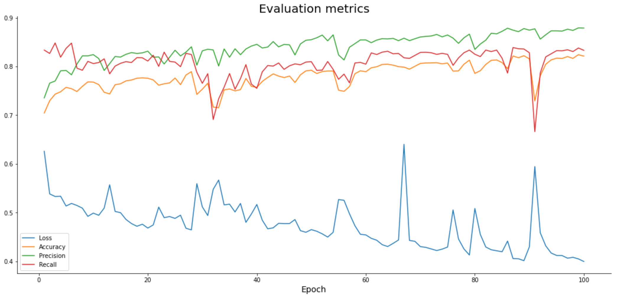
Image 8 — Model performance during training (image by author)
Accuracy, precision, and recall increase slightly as we train the model, while loss decreases. All have occasional spikes, which would hopefully wear off if you were to train the model longer.
According to the chart, you could train the model for more epochs, as there’s no sign of plateau.
But are we overfitting? Let’s answer that next.
Making predictions
You can now use the predict() function to get prediction probabilities on the scaled test data:
predictions = model.predict(X_test_scaled)
Here’s how they look like:
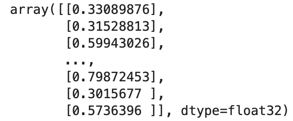
Image 9 — Prediction probabilities (image by author)
You’ll have to convert them to classes before evaluation. The logic is simple — if the probability is greater than 0.5 we assign 1 (good wine), and 0 (bad wine) otherwise:
prediction_classes = [
    1 if prob > 0.5 else 0 for prob in np.ravel(predictions)
]
Here’s how the first 20 look like:

Image 10 — Prediction classes (image by author)
That’s all we need — let’s evaluate the model next.
Model evaluation on test data
Let’s start with the confusion matrix:
from sklearn.metrics import confusion_matrix

print(confusion_matrix(y_test, prediction_classes))

Image 11 — Confusion matrix (image by author)
There are more false negatives (214) than false positives (99), so the recall value on the test set will be lower than precision.
The following snippet prints accuracy, precision, and recall on the test set:
from sklearn.metrics import accuracy_score, precision_score, recall_score


print(f'Accuracy: {accuracy_score(y_test, prediction_classes):.2f}')
print(f'Precision: {precision_score(y_test, prediction_classes):.2f}')
print(f'Recall: {recall_score(y_test, prediction_classes):.2f}')
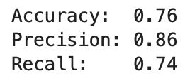
Image 12 — Accuracy, precision, and recall on the test set (image by author)
All values are somewhat lower when compared to train set evaluation:
- Accuracy: 0.82
- Precision: 0.88
- Recall: 0.83
The model is overfitting slightly, but it’s still decent work for a couple of minutes. We’ll go over the optimization in the following article.
Parting words
And that does it — you now know how to train a simple neural network for binary classification. The dataset we used today was relatively clean, and required almost zero preparation work. Don’t get used to that feeling.
There’s a lot we can improve. For example, you could add additional layers to the network, increase the number of neurons, choose different activation functions, select a different optimizer, add dropout layers, and much more. The possibilities are almost endless, so it all boils down to experimentation.
The following article will cover optimization — you’ll learn how to find the optimal learning rate and neural network architecture automatically, so stay tuned if you want to learn more.
Thanks for reading.
Stay connected
- Sign up for my newsletter
- Subscribe on YouTube
- Connect on LinkedIn

