
Part 1/6 — Introduction to GPX, exploring, and visualizing a Strava route
I love cycling, and I love using Strava to keep track of my training activities. As a data nerd, I’m a bit disappointed with their workout analysis. Sure, you can analyze speed, power, cadence, heart rate, and whatnot — depending on the sensors you have available — but what I really miss is a deep gradient analysis.
Now, a gradient in data science and cycling don’t necessarily represent the same thing. In cycling, it’s basically the slope of the surface you’re riding on. Being a tall and somewhat heavy rider I find hills challenging, so a deeper gradient analysis would be helpful. For example, I’d like to see how much distance I’ve covered between 3 and 5 percent grade, how much was above 10, and everything in between. You get the point.
Strava doesn’t offer that functionality, so I decided to do the calculations from scratch using my Python skills.
Join me in a 6 article mini-series that will kick of with a crash course in GPX file format and end in a dashboard that displays your training data in more depth than Strava.
Don’t feel like reading? Watch my video instead:
You can download the source code on GitHub.
GPX Crash Course for Data Science
Strava lets you export your workouts and routes in GPX file format. Put simply, GPX stands for GPS Exchange Format, and it’s nothing but a text file with geographical information, such as latitude, longitude, elevations, tracks, waypoints, and so on.
An exported Strava route GPX file has many points taken at different times, each containing latitude, longitude, and elevation. In simple terms, you know exactly where you were and what was your altitude. This is essential for calculating gradients and gradient ranges, which we’ll do in a couple of articles.
If you’re following along, head over to Strava and download any of your saved routes (Export GPX button):
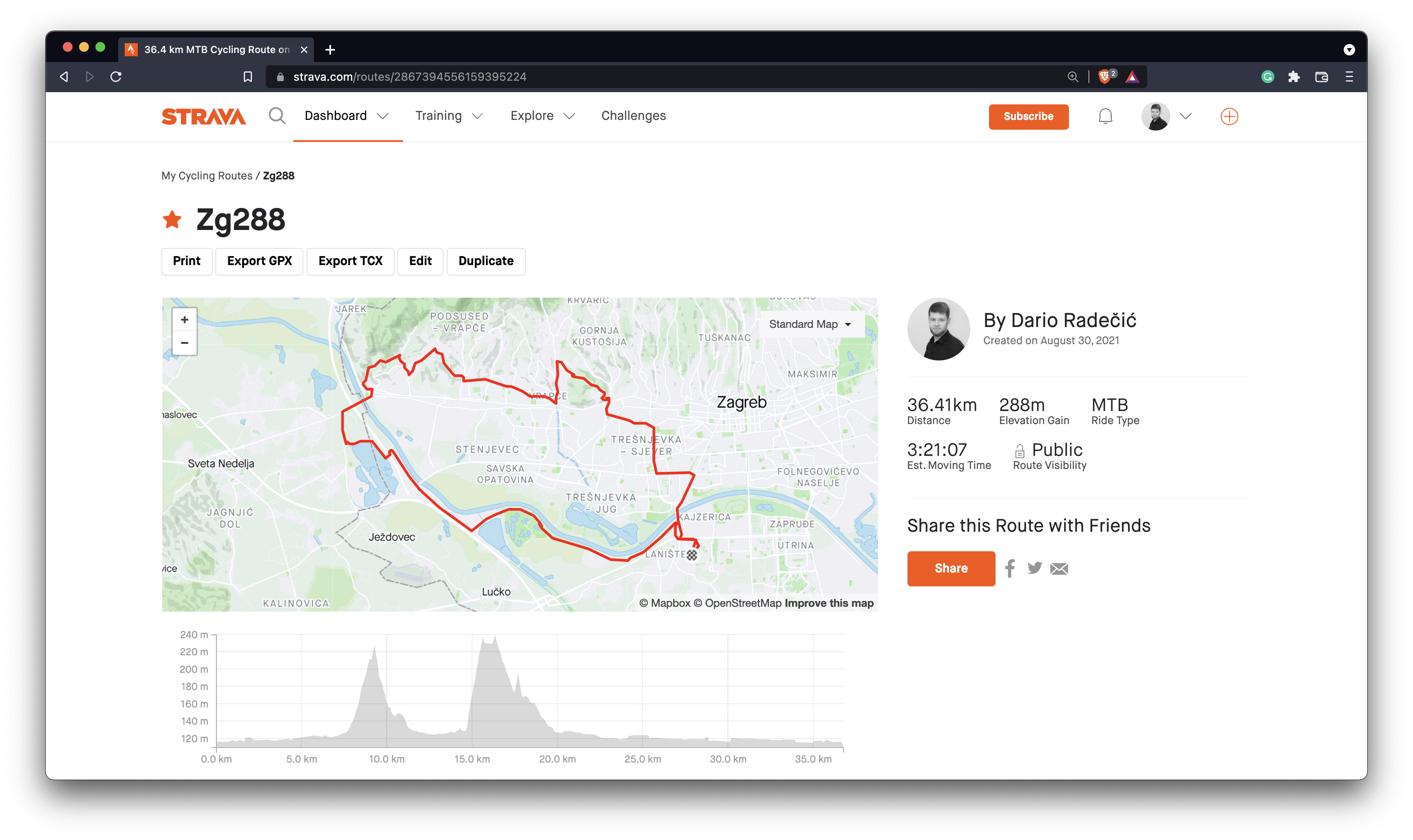
Image 1 — A roundtrip Strava route in Zagreb, Croatia (image by author)
Creating routes requires a paid Strava subscription, so for safety concerns I won’t share my GPX files with you. Use any GPX file from your routes or the training log. If you’re not using Strava, simply find a sample GPX file online, it should still work.
Got the GPX file ready? Awesome — let’s see how to read it with Python next.
How To Read GPX Files With Python
You’ll need a dedicated gpxpy package to read GPX with Python. Install it with Pip:pip install gpxpy
You can now launch Jupyter or any other code editor to get started. First things first, let’s get the library imports out of the way:
import gpxpy
import gpxpy.gpx

import pandas as pd
import matplotlib.pyplot as plt
plt.rcParams['axes.spines.top'] = False
plt.rcParams['axes.spines.right'] = False
Use Python’s context manager syntax to read and parse a GPX file:
with open('../src_code/Zg288.gpx', 'r') as gpx_file:
    gpx = gpxpy.parse(gpx_file)
Please note you’ll have to change the path to match your system and GPX file name. If everything went well, you should have the file now available in Python.
But what’s inside? Let’s see:
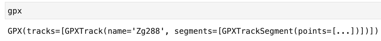
Image 2 — Contents of the GPX file (image by author)
It’s a specific GPX object with the track name and segment, where each segment contains data points (latitude, longitude, and elevation). We’ll dive deeper into these in the following section, but first, let’s explore a couple of useful functions.
For example, you can extract the total number of data points in a GPX file:
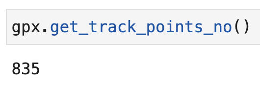
Image 3 — Total number of data points in the GPX file (image by author)
There are 835 points in total, each containing latitude, longitude, and elevation data. That will come useful later.
You can also get the altitude range:
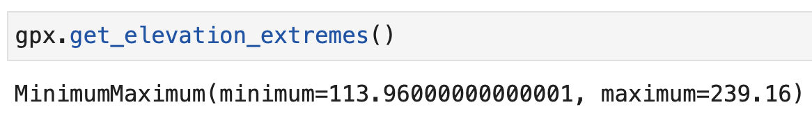
Image 4 — Minimum and maximum altitudes (image by author)
In plain English, this means that the lowest point of the ride is 113,96 meters above sea level, while the highest is at 239,16 meters.
You can also extract the total meters of elevation gained and lost:
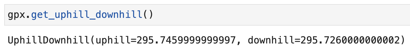
Image 5 — Total elevation gained and lost (image by author)
My route represents a roundtrip, so it’s expected to see identical or almost identical values. Lastly, you can display the contents of your GPX file in XML format:
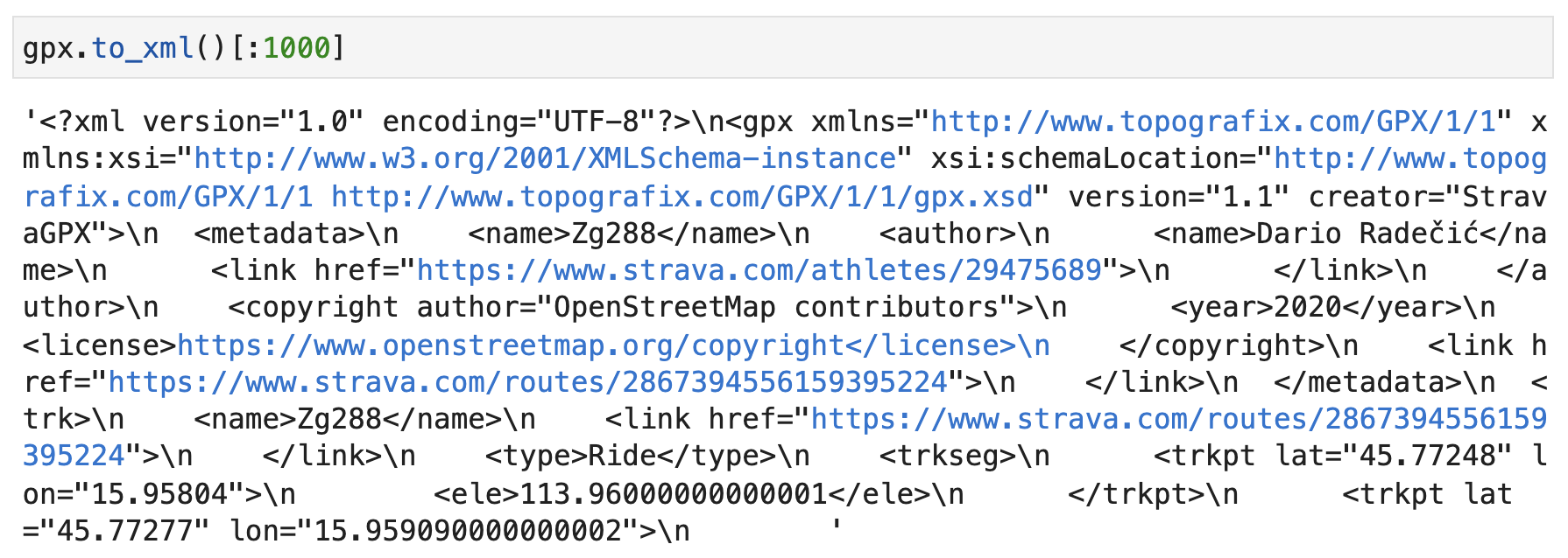
Image 6 — GPX file in XML format (image by author)
It’s not super-readable, but it might come in handy if you have an XML processing pipeline.
And that does it for the basics. Next, you’ll see how to extract individual data points and convert them into a more readable format — Pandas DataFrame.
How To Analyze GPX Files With Python
You can check how many tracks your GPX file has by running len(gpx.tracks). Mine has only one, and I can access it with Python’s list indexing notation:
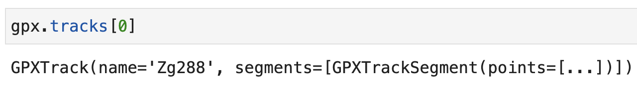
Image 7 — Accessing a single track (image by author)
We don’t care for the name of the track, as it’s arbitrary in this case. What we do care about are the segments. As with tracks, my GPX file has only one segment on this track. Here’s how to access it:
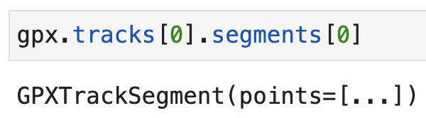
Image 8 — Accessing a single segment (image by author)
And now you can access individual data points by accessing the points array. Here are the first ten for my route:
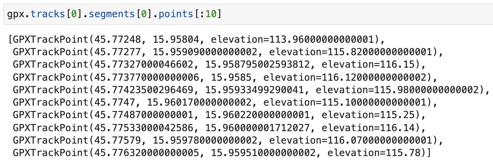
Image 9 — Accessing individual data points (image by author)
That’s all we need to have some fun. You’ll now see how to extract individual data points from the GPX file:
route_info = []

for track in gpx.tracks:
    for segment in track.segments:
        for point in segment.points:
            route_info.append({
                'latitude': point.latitude,
                'longitude': point.longitude,
                'elevation': point.elevation
            })
It’s not the prettiest code you’ve ever seen, but gets the job done. Let’s print the first three entries to verify we did everything correctly:
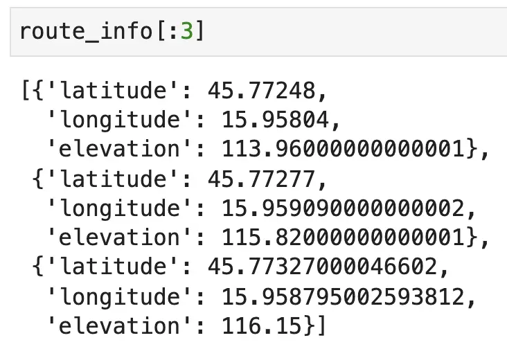
Image 10 — Extracted data points as a list of dictionaries (image by author)
Do you know what’s extra handy about a list of dictionaries? You can convert it to a Pandas DataFrame in a heartbeat:
route_df = pd.DataFrame(route_info)
route_df.head()
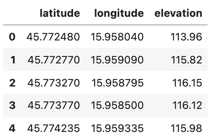
Image 11 — Extracted data points as a Pandas DataFrame (image by author)
You have to admit — that was pretty easy! We’ll need this dataset in the following articles, so let’s dump it into a CSV file:
route_df.to_csv('../data/route_df.csv', index=False)
That’s all for the basic analysis and preprocessing we’ll do today. I’ll also show you how to visualize this dataset with Matplotlib — just to see if we’re on the right track.
How To Visualize GPX Files With Python and Matplotlib
We’ll work on route visualization with Python and Folium in the following article, but today I want to show you how to make a basic visualization with Matplotlib. You won’t see the map, sure, but the location points should resemble the route from Image 1.
Hint: don’t go too wide with the figure size, as it would make the map look weird.
Copy the following code to visualize the route:
plt.figure(figsize=(14, 8))
plt.scatter(route_df['longitude'], route_df['latitude'], color='#101010')
plt.title('Route latitude and longitude points', size=20);
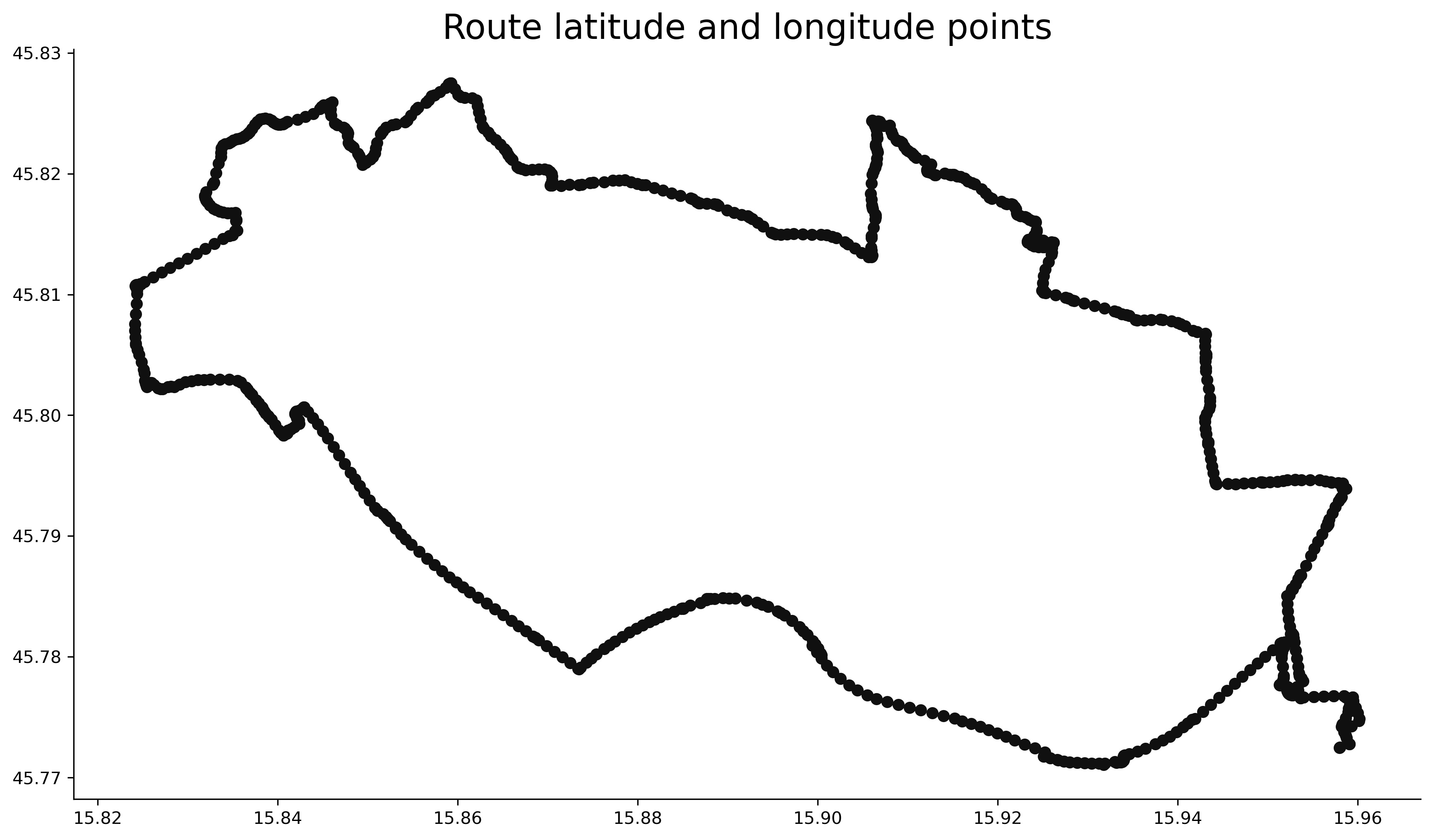
Image 12 — Route visualization with Matplotlib (image by author)
And who would tell — it’s identical to what we had in Image 1, not taking the obvious into account. You’ll learn all about map and route visualization in the following article.
Conclusion
And there you have it — you’ve successfully exported a GPX route/training file from Strava, parsed it with Python, and extracted key characteristics like latitude, longitude, and elevation. It’s just the tip of the iceberg, and you can expect to learn more applications of programming and data science in cycling in the upcoming articles.
Thanks for reading, and stay tuned for more!
Stay connected
- Sign up for my newsletter
- Subscribe on YouTube
- Connect on LinkedIn